笔记链接:GAMES101: 现代计算机图形学入门-幕布链接
2020 年春季学期(在线直播),课程录像会在 Bilibili 网站 更新。
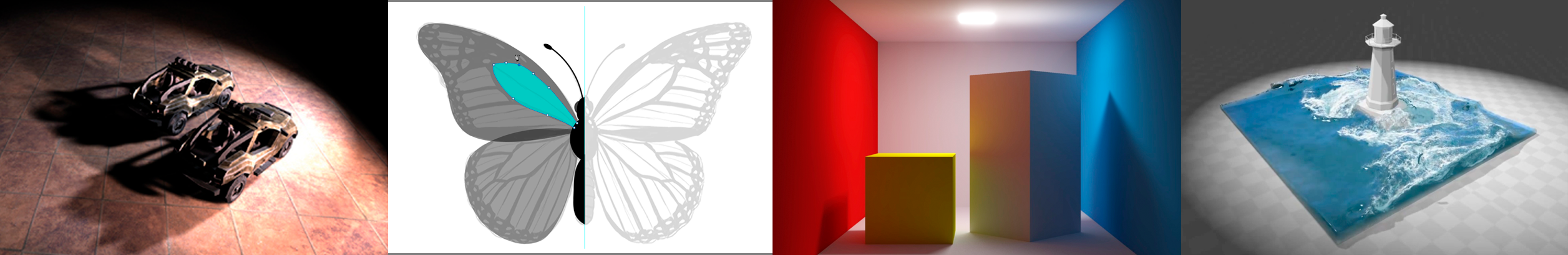
光栅化成像 [实时软阴影 (NVIDIA)]
几何表示 [Adobe Photoshop 中的钢笔工具]
光线传播理论 [光子映射 (Jensen)]
动画与模拟 [流体模拟 (Muller)]
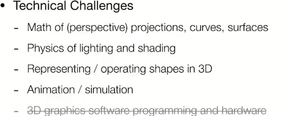
本课程将全面而系统地介绍现代计算机图形学的四大组成部分:(1)光栅化成像,(2)几何表示,(3)光的传播理论,以及(4)动画与模拟。每个方面都会从基础原理出发讲解到实际应用,并介绍前沿的理论研究。通过本课程,你可以学习到计算机图形学背后的数学和物理知识,并锻炼实际的编程能力。
顾名思义,作为入门,本课程会尽可能的覆盖图形学的方方面面,把每一部分的基本概念都尽可能说清楚,让大家对计算机图形学有一个完整的、自上而下的全局把握。全局的理解很重要,学完本课程后,你会了解到图形学不等于 OpenGL,不等于光线追踪,而是一套生成整个虚拟世界的方法。从本课程的标题,大家还可以看到“现代”二字,也就是说,这门课所要给大家介绍的都是现代化的知识,也都是现代图形学工业界需要的图形学基础。
本课程与其它图形学教程还有一个重要的区别,那就是本课程不会讲授 OpenGL,甚至不会提及这个概念。本课程所讲授的内容是图形学背后的原理,而不是如何使用一个特定的图形学 API。在学习完这门课的时候,你一定有能力自己使用 OpenGL 写实时渲染的程序。另外,本课程并不涉及计算机视觉、图像视频处理、深度学习,也不会介绍游戏引擎与三维建模软件的使用。
具体课程内容请参见课程大纲。
1. 第一讲-什么是图形学
1.1. 是什么
1.2. 应用
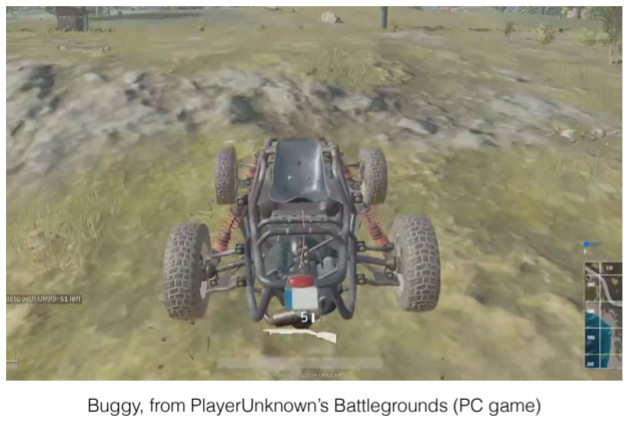
- video game-画面好不好 在图形学里面就看亮不亮 全局光照
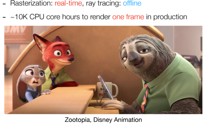
- movie-特效(最常见的图形学应用)
- Animations-渲染、模拟
- design-模拟碰撞、曲面造型、渲染 ,工业设计和家装设计等
- visualization
- VR
- digital illustration
- simulation
- GUI
1.3. 为什么

1.4. Course topic
1.4.1. Rasterization
1.4.2. Curves and meshes
1.4.3. Ray tracing

1.4.4. Animation/Simulation
1.5. 图形学与视觉的区别

2. 第二讲-向量与线性代数
2.1. 图形学的依赖
- 基础数学、基础物理、信号处理、数值分析、美学
2.2. 向量
2.2.1. 向量的归一化
2.2.2. 和
2.2.3. cartesian coordinates
便于表示及计算长度,图形学中默认向量为列向量或用转置写成行向量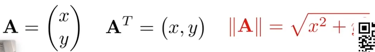
2.2.4. 乘
2.2.4.1. 点乘
- 结果为标量,在图形学中可以用来计算向量之间的夹角
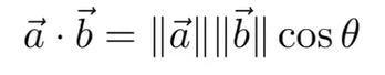
   - 满足交换律、分配律、结合律

    - 笛卡尔坐标系下的点乘

    - 在图形学中的应用

      - 在图形学中可以用来计算向量之间的夹角
      - 一个向量在另一个向量上的投影
2.2.4.2. Cross product
- 升维
- 在构建坐标系中很有用 ,a x b得到的向量 垂直于a、b
- 应用
- 判定左和右
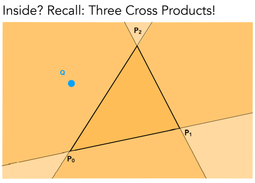
- 判断内和外
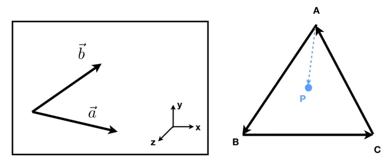
- 正交坐标系
2.3. 矩阵
- 结合律 分配律
- 向量为特殊的m*1矩阵
3. 第三讲-transform
3.1. why
- modeling
- viewing
3.2. 2d变换
3.2.1. scale缩放(均匀与非均匀缩放)
3.2.2. reflection 镜像操作
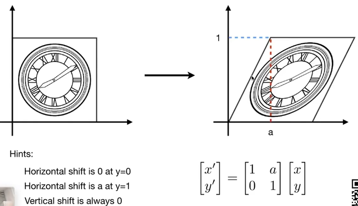
3.2.3. shear matrix 切片矩阵
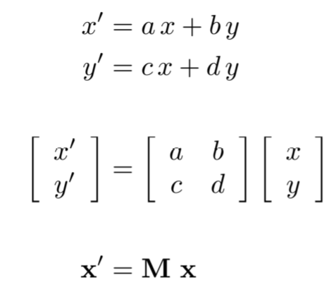
3.2.4. rotation matrix
3.2.5. linear transform = matrices
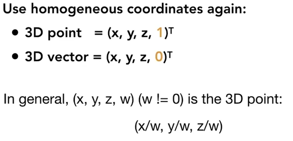
3.3. homogeneous coordinates
3.3.1. why
对于translation变换 发现无法用矩阵的形式表示,必须加上平移的操作,因为平移不是线性变换. 但是我们又不想将其当作是一种特殊的变换,因此寻求一种新的统一的方式

3.3.2. solution:
homogeneous coordinates
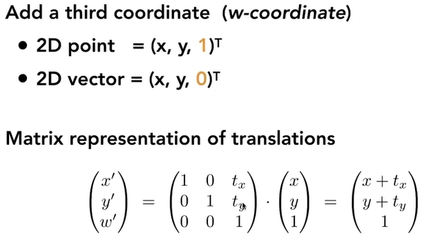
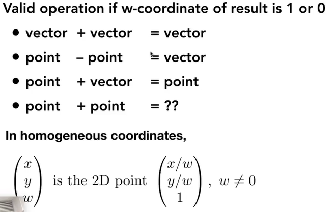
2d point 和 2d vector区别对待 是考虑到向量的平移不变性point + point 为这两个点的中点
3.3.3. affine transformation
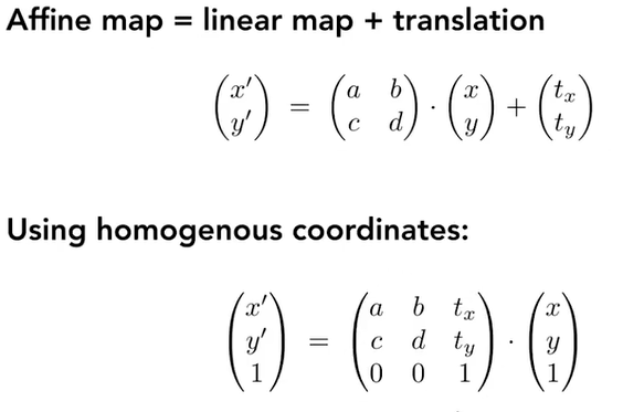
任何放射变换都可以用齐次坐标表示只有在二维仿射变换下最后一行才为001,其他有不同的情况
3.4. inverse transform
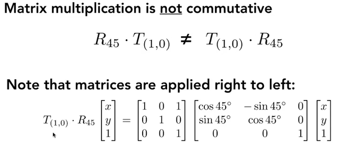
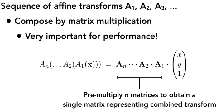
3.5. composite transform变换的组合
变换的顺序是很重要的,例如先平移后旋转、先旋转后平移是不一样
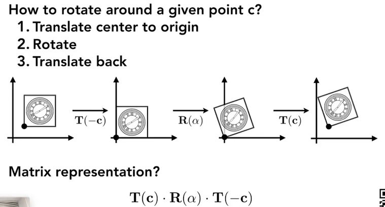
3.6. decomposing complex transform
3.7. 3D transformations(包括部分第四讲内容)
3.7.1. 三维的变换也是先应用线性变换后应用平移变换
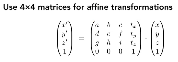
3.7.2. 三维的缩放和平移 旋转
3.7.2.1. 缩放和平移
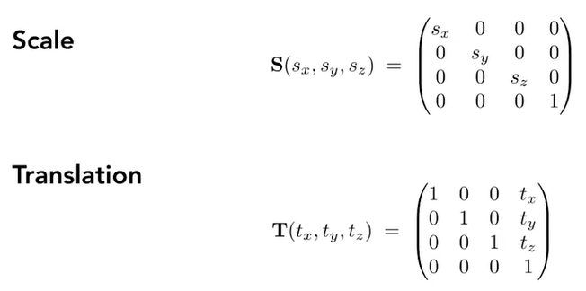
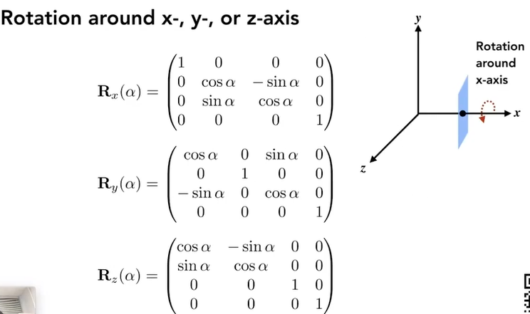
3.7.2.2. 3D旋转
注意观察绕y轴的旋转矩阵 、循环对称的性质。这是因为二位平面定义时,逆时针实际是在三维从z正向看,因此3维绕y旋转,逆时针实际是z向x转,但是旋转矩阵的行列对应关系是x向z转,取逆(转置)就得到了
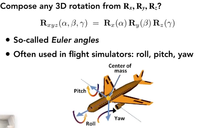
3.7.2.2.1. 欧拉角
用欧拉角的形式来将任意旋转矩阵分解为绕xyz轴的旋转组合
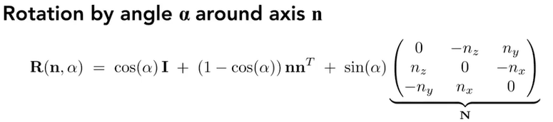
3.7.2.2.2. Rodrigues’ rotation formula
绕任意轴,先将轴的起点平移到原点 旋转,在平移回去 2.N,在计算向量叉乘的时候,用矩阵的表示方式
证明
四元数目的是为了方便旋转的差值计算
3.8. 补充内容
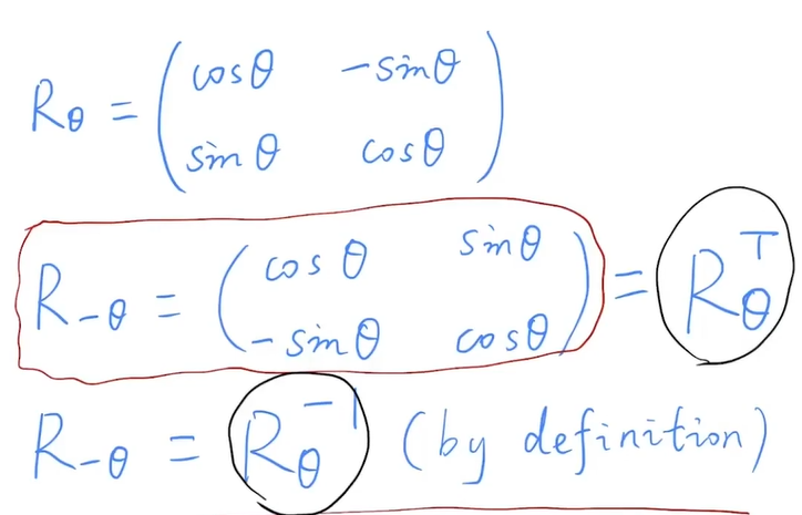
旋转矩阵的逆等于旋转矩阵的转置,我们逆等于它的转置的矩阵称之为正交矩阵
4. 第四讲-transformation Cont.
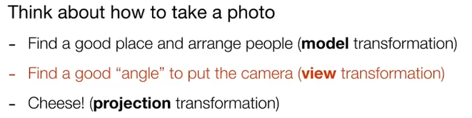
4.1. viewing transformation
4.1.1. view / camera transformation
4.1.1.1. MVP
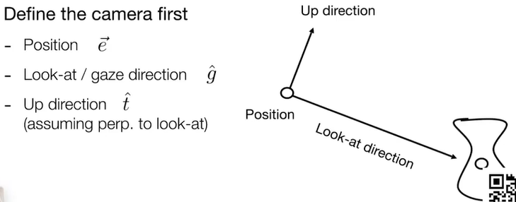
4.1.1.2. 相机的定义,如何做view transformation
4.1.1.3. key observation
当相机与物体之间不存在相对运动时候,照片是一样的,因此可以定义一个坐标系。简化操作,这里是右手坐标系
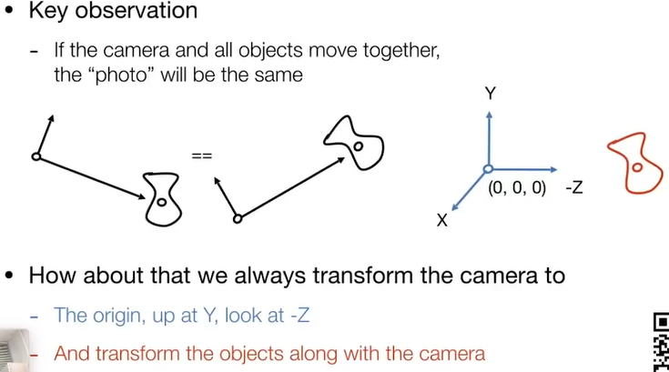
4.1.1.4. 将任意位置摆放的相机转为标准的摆放
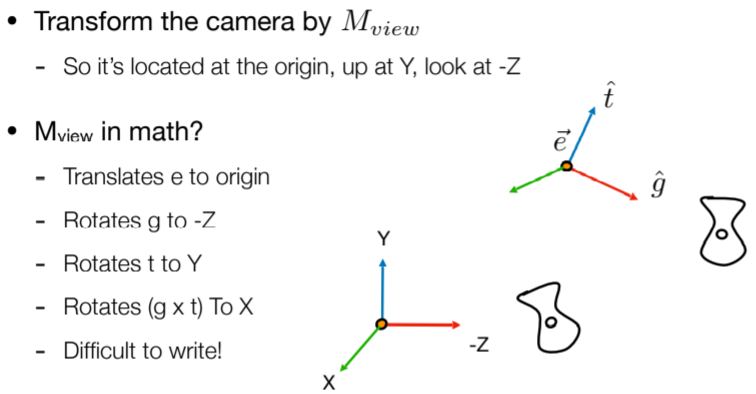
4.1.1.5. 数学表达
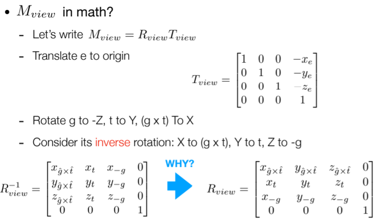
    - 这里是先平移再旋转
    - 假如将任意轴旋转到某个标准轴,如001,会很难,那么将001旋转到任意轴,会简单很多,因此这里用了逆的概念
    - 旋转矩阵是正交矩阵,因此它的逆等于它的转置
4.1.1.6. summary
这里物体随着相机一块运动

4.1.2. projection transformation
4.1.2.1. 二者差别

4.1.2.2. orthographic projection
4.1.2.2.1. 简单的理解
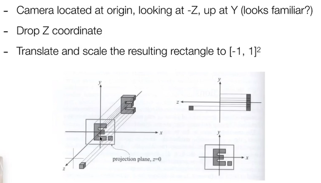
4.1.2.2.2. 方向的通用定义
这里f(far)<n(near),因为我们是看向-z方向,使得near和far并不直观,这也就是在OpenGL的API中使用左手坐标系的原因,看起来更直观。


4.1.2.2.3. transformation matrix。这里2是因为缩放到(-1,1)之间,长度为2

4.1.2.3. perspective projection
近大远小,图形学中应用最广泛的投影,平行线会相较于一点
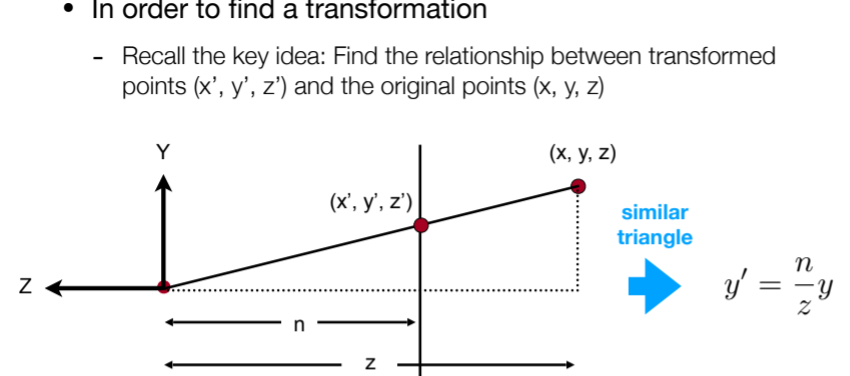
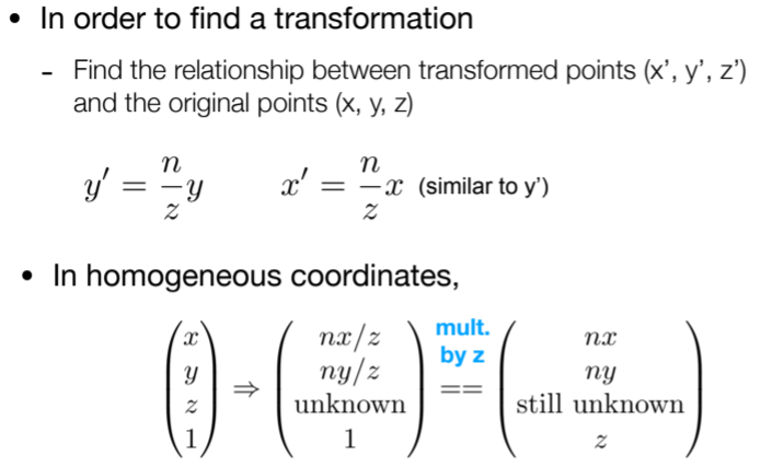
4.1.2.3.1. 回忆知识点!!!

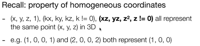
4.1.2.3.2. 怎么做透视投影,拆分思路?规定近平面四个点不变,原平面z值不变
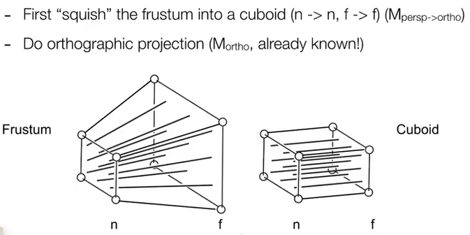
- 将投影squish为正视。注意这里用到了上面说的两个不变条件
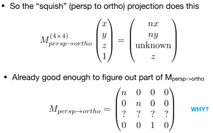
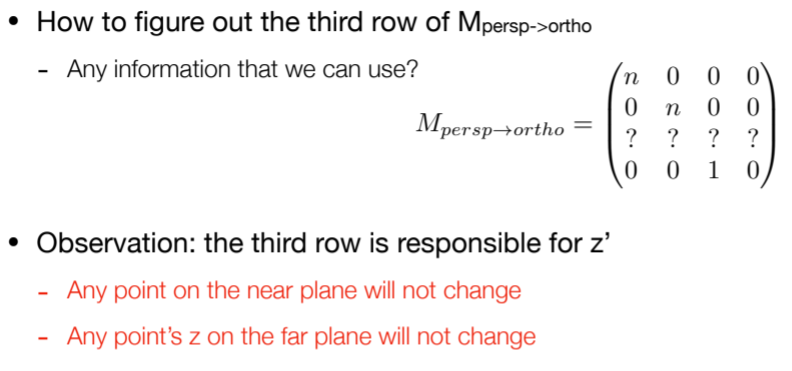

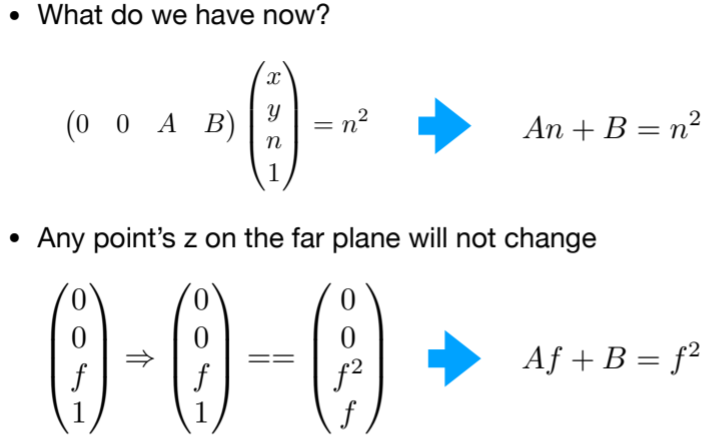
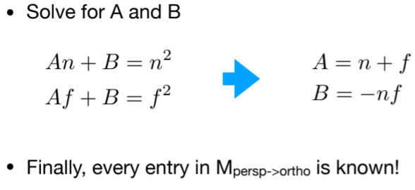
- Do orthographic projection (Mortho) to finish

- 对于near和far平面 他们的z成什么样一种变化,变小 大还是不变,根据计算的投影矩阵得到是变小
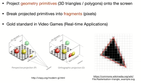
5. 第五讲-光栅化rasterization 1(triangles)
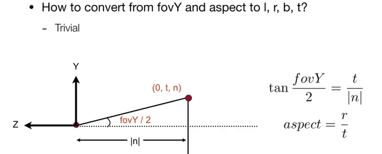
5.1. 透视投影
5.1.1. 近平面:长宽比/垂直可视角度
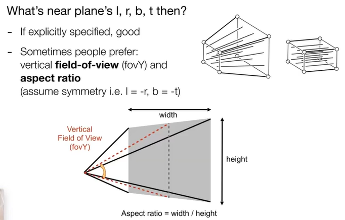
5.1.2. fovY与l、r、b、t关系
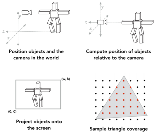
5.1.3. MVP之后 需要将canonical cube to screen-光栅化
5.1.3.1. 定义屏幕空间
5.1.3.2. 变换到xy平面

5.1.3.3. rasterizing triangles into pixels
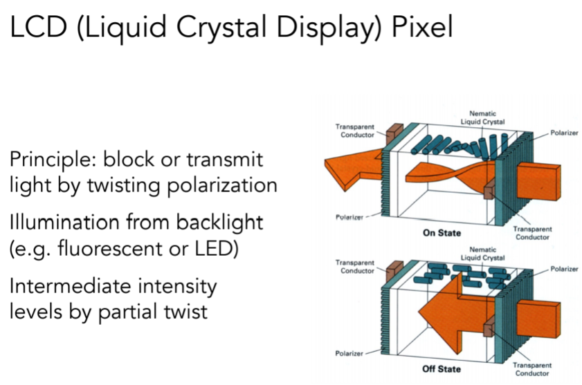
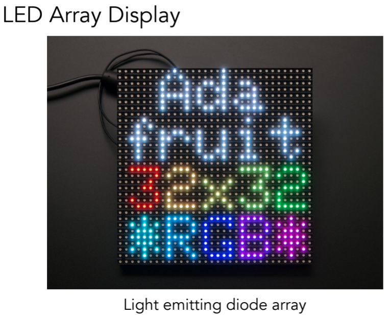
5.1.3.3.1. 显示设备
5.1.3.3.2. Rasterization: Drawing to Raster Displays
- mesh
- Polygon Meshes多边形网格
- triangle meshes-why
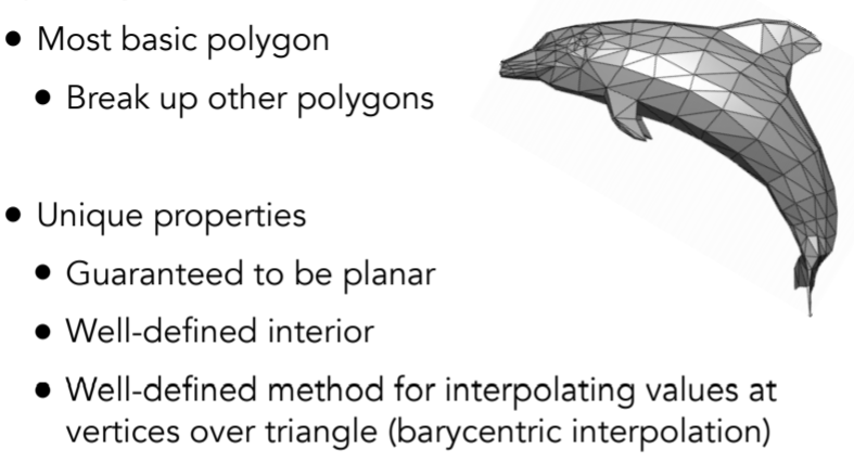
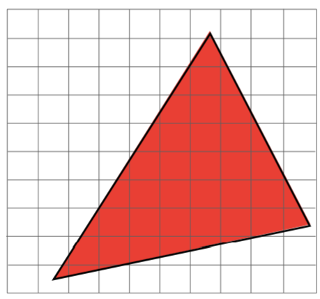
- triangle 与屏幕像素之间的关系
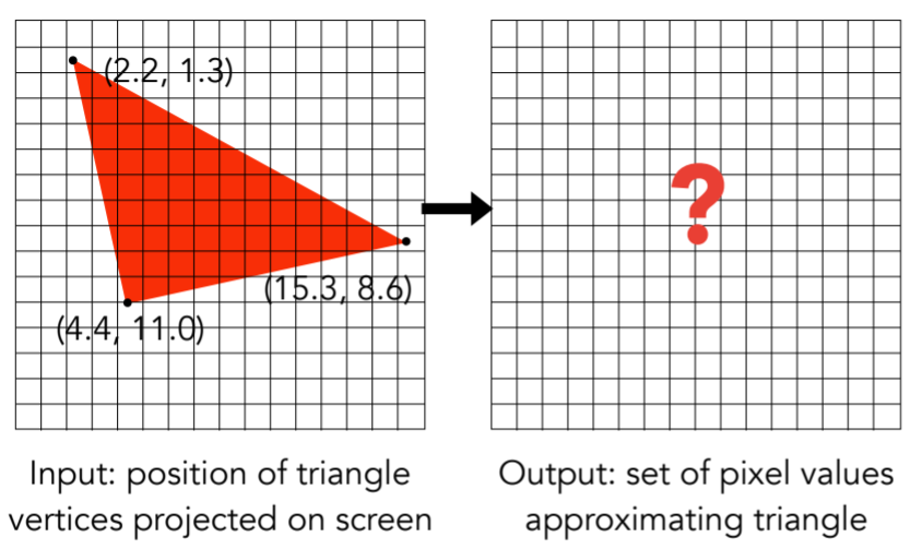
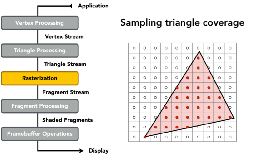
        - a simple approach:sampling

          - Rasterization As 2D Sampling
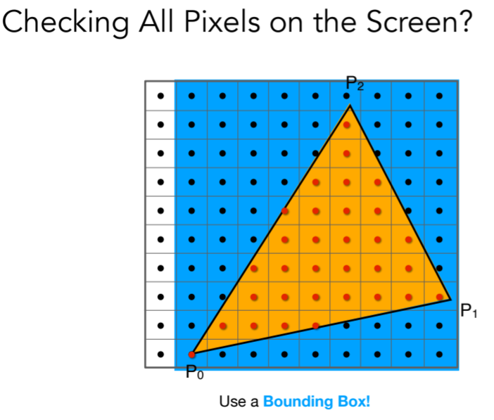
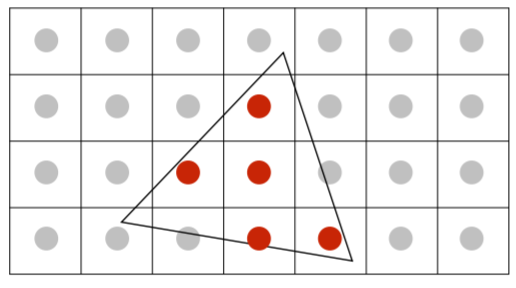
- Sample If Each Pixel Center Is Inside Triangle
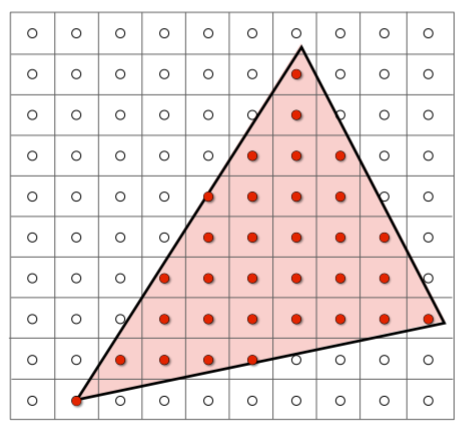
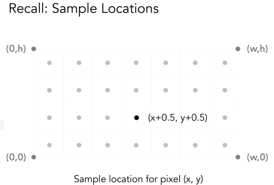
- 要注意的是,像素是i,j表示,但是像素的中心是在i+0.5,j+0.5的
- 接下就是判断点是否在三角形内部:某一顺逆时针方向上的向量叉乘
          - 这样全部的便利,似乎很慢,因此改进型

            - 包围盒AABB
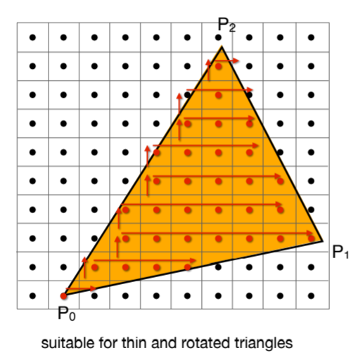
- Incremental Triangle Traversal (Faster?)
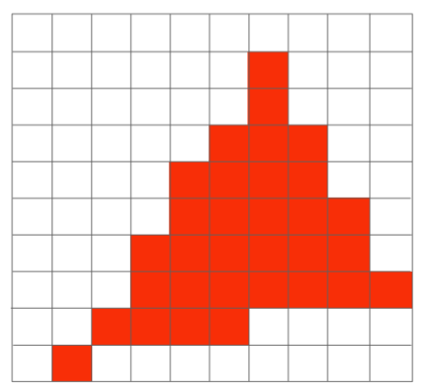
5.1.3.3.3. Rasterization on Real Displays
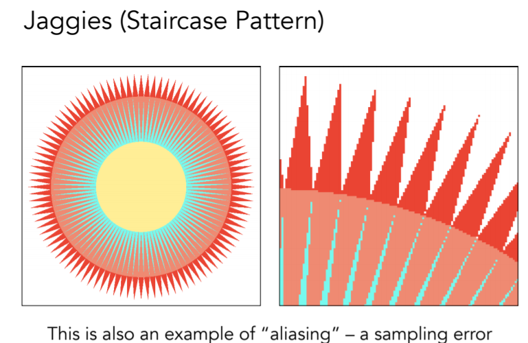
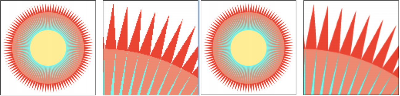
- Jaggies锯齿问题 走样
6. 第六讲-光栅化2(反走样和z-缓冲Antialiasing and z-buffering)
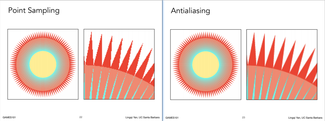
6.1. Antialiasing
6.2. Sampling theory
6.2.1. 回忆内容
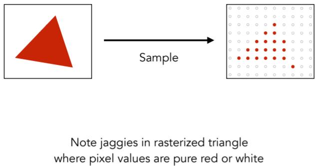
像素中心是否在三角形内部,但是这样得到的结果存在锯齿,学名走样
6.2.2. 采样理论
6.2.2.1. 采样在图形学中广泛存在,采样可以发生在不同的位置、时间
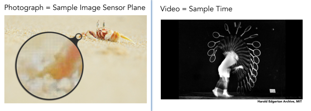
6.2.2.1.1. 采样产生的问题也是广泛存在的
- 锯齿
- 图片中的摩尔纹

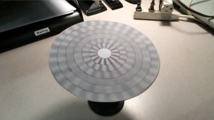
- Wagon Wheel Illusion (False Motion)
- 总结

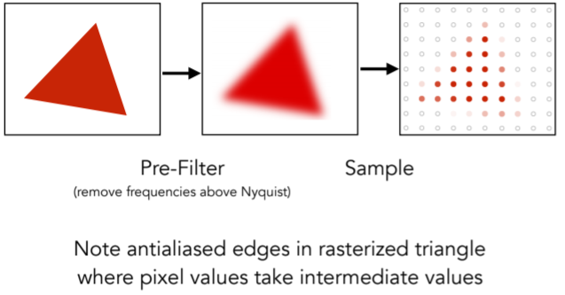
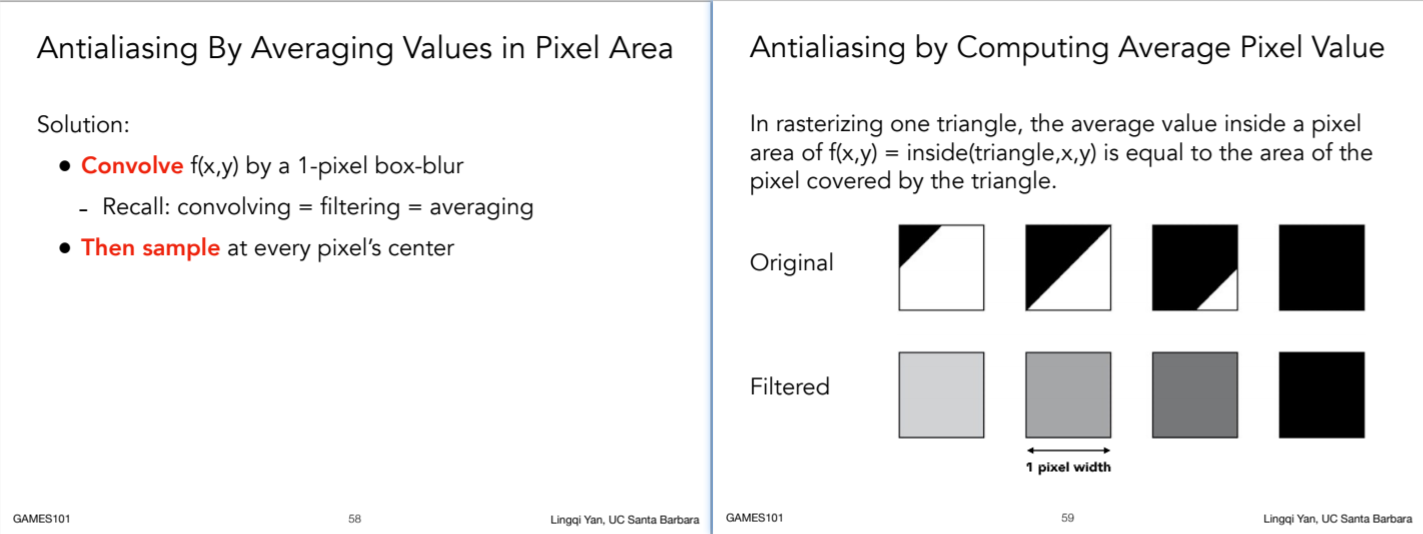
6.2.2.2. Antialiasing Idea: Blurring (Pre-Filtering) Before Sampling,即先模糊再采样,反之不行
6.2.2.2.1. 反采样原理
- Rasterization: Point Sampling in Space

- Rasterization: Antialiased Sampling
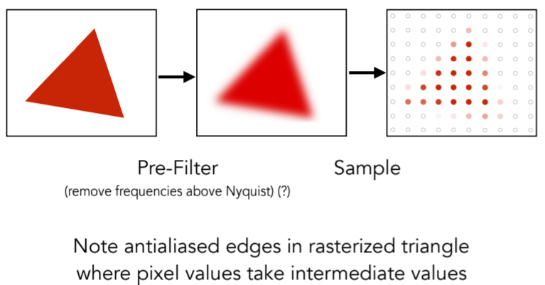
- 二者对比
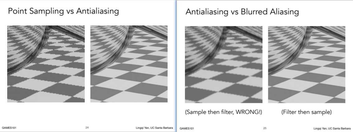
6.2.2.2.2. 为什么欠采样会引入走样 / 为什么 pre-filtering then sampling can do antialiasing
相关知识:
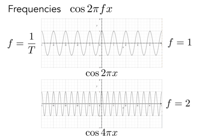
    - 频域Frequency Domain

      - 频率f 周期T
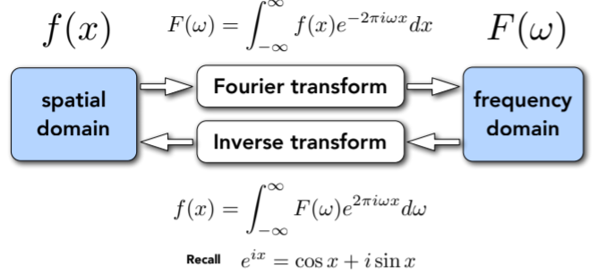
- Fourier Transform(任一周期性函数都是正弦/余弦函数得线性组合)
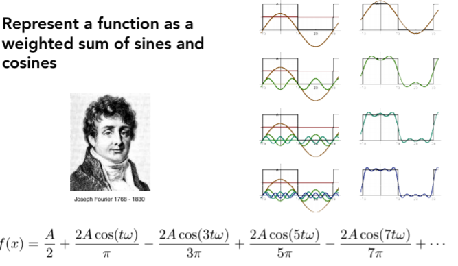
- Fourier Transform Decomposes A Signal Into Frequencies傅里叶变换将信号分解成频率,注意时域与频域之间得变换
- Higher Frequencies Need Faster Sampling
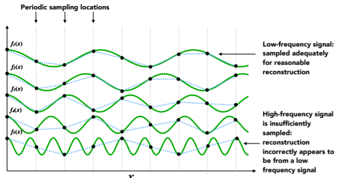
- Undersampling Creates Frequency Aliases(两种不同频率得函数 得到了同一个采样结果,这就是走样)

- Filtering(= Getting rid of certain frequency contents)
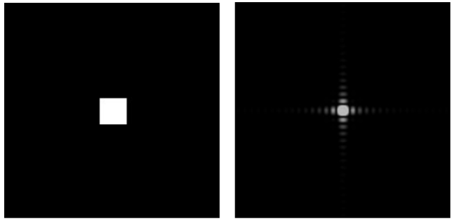
- Visualizing Image Frequency Content (注意观察)时域图片经过傅里叶变换得到频域图

            - 观察一:频谱图包含低频(中心定义为最低频区域)、高频信息(周围定义为高频),也就是从中心到周围越来越高,包含的信息用亮度来表示,这个图中就是说图片中低频信息很多
            - 观察二:水平/竖直高亮条:在分析信号得时候,认为信号是周期性重复出现得,而对于照片来讲,我们将其水平和竖直周期性延拓,那么边界得位置会发生剧烈得变化,产生高频信息

          - Filter Out Low Frequencies Only (Edges),只保留得边界信息

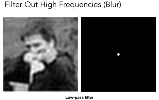
- Filter Out High Frequencies (Blur) 低通之后丢失边界信息 变得模糊
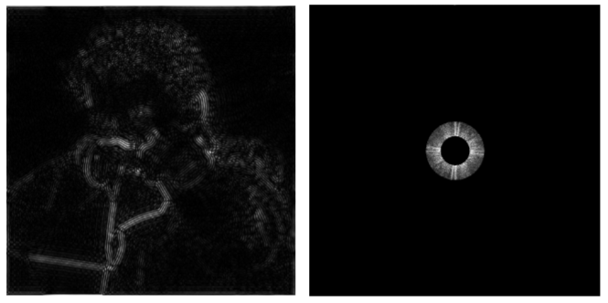
          - 带通滤波

            - Filter Out Low and High Frequencies

- Filter Out Low and High Frequencies
        - Filtering = Convolution(= Averaging)

          - Convolution 滑动窗口

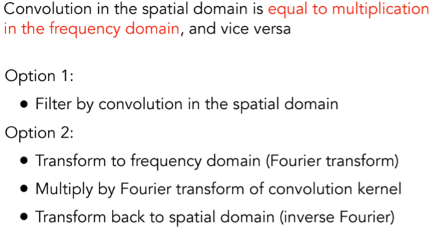
- Convolution Theorem时域卷积=频域乘积,时域乘积=频域卷积。两种时域卷积得方式
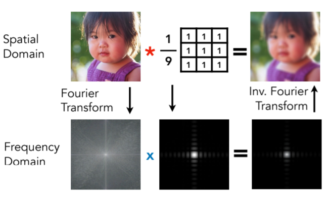
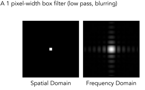
- Box Filter
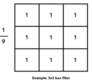
- Box Function = “Low Pass” Filter
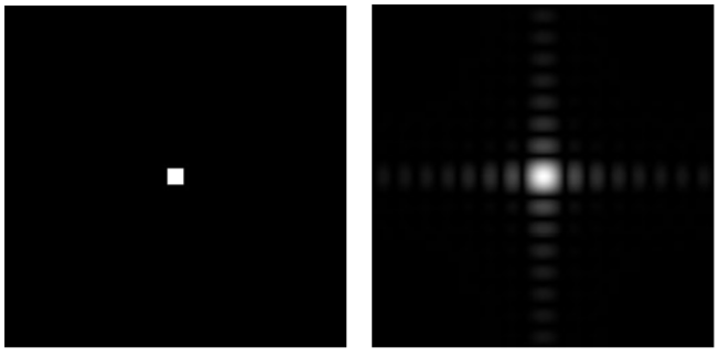
- Wider Filter Kernel = Lower Frequencies 更大得卷积核 更模糊
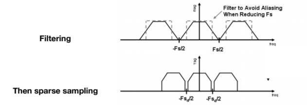
        - Sampling = Repeating Frequency Contents

          - Sampling = Repeating Frequency Contents
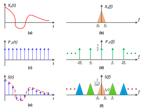
            - 用频率得角度去看采样,同时时域采样等于频域得周期性延拓

          - Aliasing = Mixed Frequency Contents
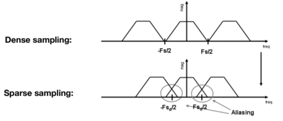
- 对于冲激函数,频域间隔等于时域间隔得倒数,因此越稀疏,采样间隔越宽,再频域则越窄,导致走样
6.2.2.2.3. Antialiasing in practice
- How Can We Reduce Aliasing Error?
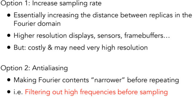
- Antialiasing = Limiting, then repeating
- Regular Sampling
- Antialiased Sampling
- A Practical Pre-Filter
6.2.2.2.4. Antialiasing By Supersampling(MSAA)
- Point Sampling: One Sample Per Pixel
- Supersampling
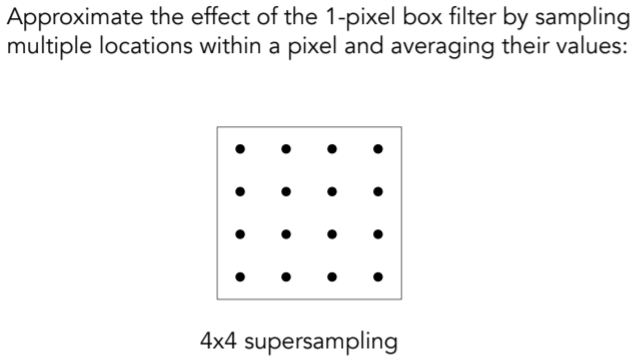
- step1:Take NxN samples in each pixel
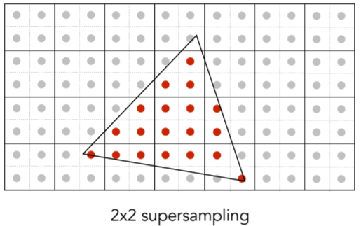
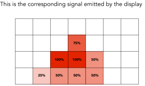
- Step 2:Average the NxN samples “inside” each pixel.
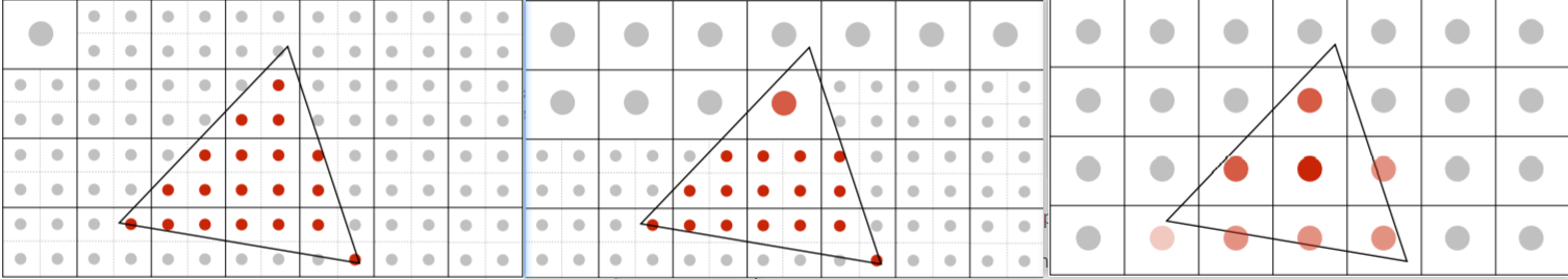
- Result
- attention:这只是对反走样得近似,第一步是对信号得模糊,supersample只是得到近似三角形得覆盖,并没有增加分辨率
6.2.2.3. 总结:
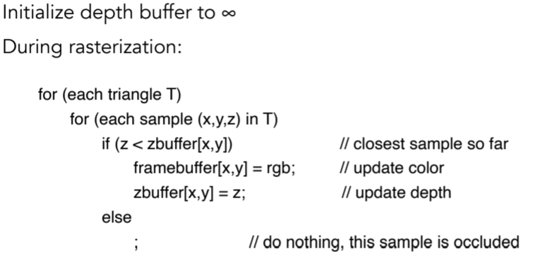
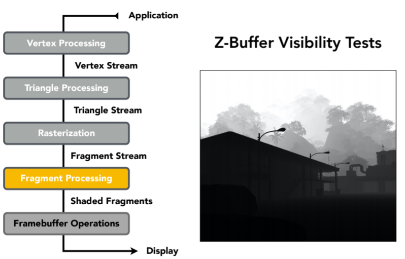
6.3. visibility / occlusion(第七讲视频)– Z-Buffering
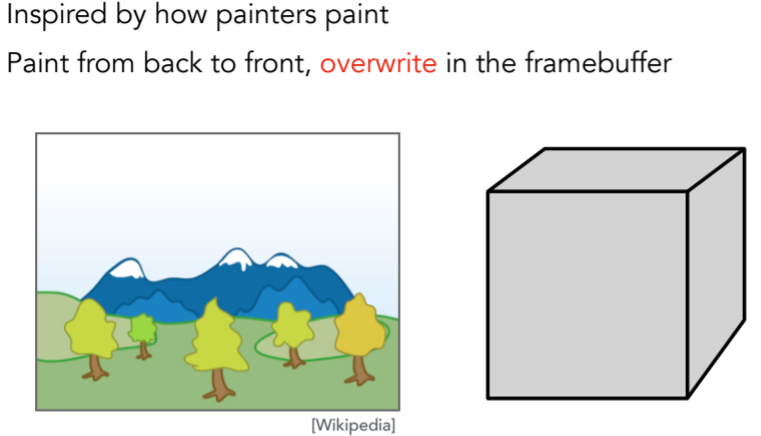
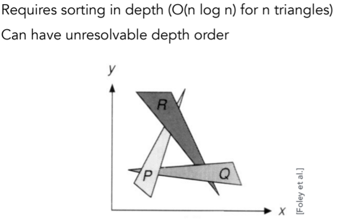
6.3.1. Painter’s Algorithm画家算法(特指油画)
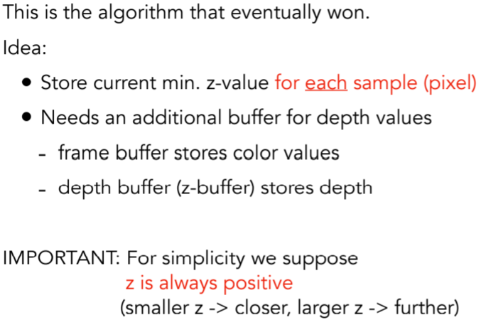
6.3.2. Z-buffer 注意这里的frame buffer 和depth buffer的作用。并且有一个假设z是正值;是对像素的排序,而不是对三角形的远近排序
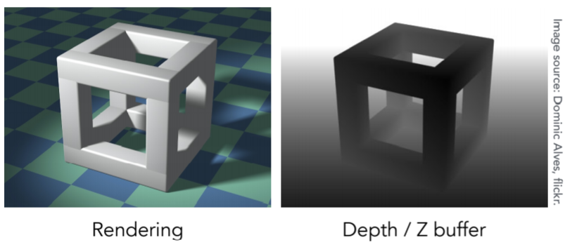
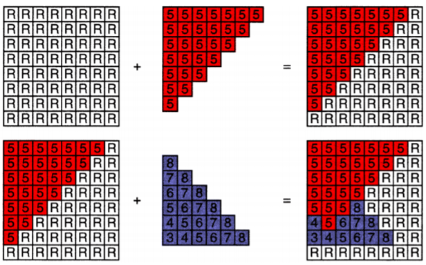
6.3.3. z-buffer的例子
6.3.4. z-buffer算法;每轮绘制都有深度计算的更新
6.3.5. z-buffer复杂度
6.3.5.1. Complexity
- O(n) for n triangles (assuming constant header-imgage)
- How is it possible to sort n triangles in linear time?: 因为每次只比较记录一次最小值,不用排序
6.3.5.2. Drawing triangles in different orders? :与顺序无关
6.3.5.3. Most important visibility algorithm
Implemented in hardware for all GPUs
6.3.5.4. 在MSAA中 需要对每一个supersample得到的采样点都做Z-buffer
7. 第七讲-Shading 1 (Illumination, Shading and Graphics Pipeline)
7.1. 前面只是总结,引子
7.2. Shading:definition
7.2.1. The darkening(明暗) or coloring of an illustration or diagram with parallel lines or a block of color.
7.2.2. The process of applying a material to an object.
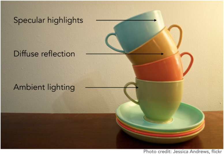
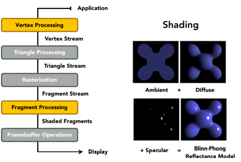
7.3. A Simple Shading Model (Blinn-Phong Reflectance Model)
7.3.1. Perceptual Observations高光,漫反射,环境光
7.3.2. Shading is Local很关键的一个点,局部局部
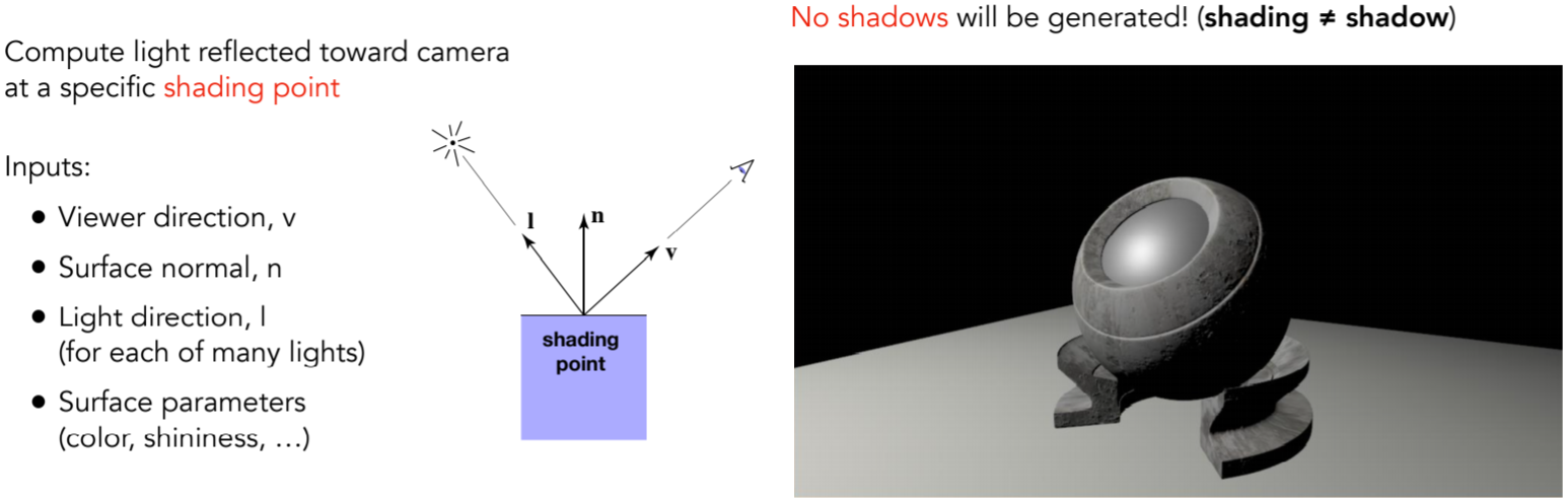
为什么l向量不从光源出发?不引入光源结构的前提下,只从着色点出发,简化模型,但是这也存在局限性,如右图
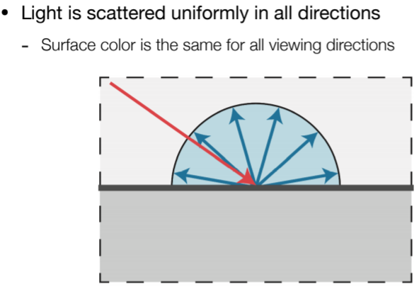
7.3.3. Diffuse Reflection
7.3.3.1. Light is scattered uniformly in all directions均匀性
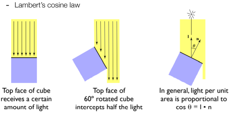
7.3.3.2. But how much light (energy) is received? 考虑的是单位面积接收到的能量,其实四季的变化的原因就在于获取不同季节内获得的太阳能量的多少。
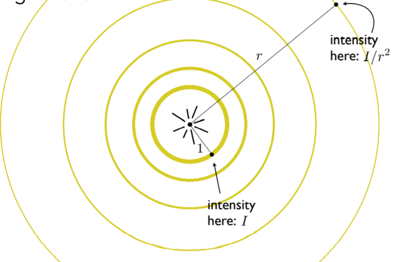
7.3.3.3. Light Falloff,同时也要考虑到光的衰减。点光源某一时刻集中于一个球壳上,考虑到能量守恒,必然导致越大的球壳上 某一点越衰减。
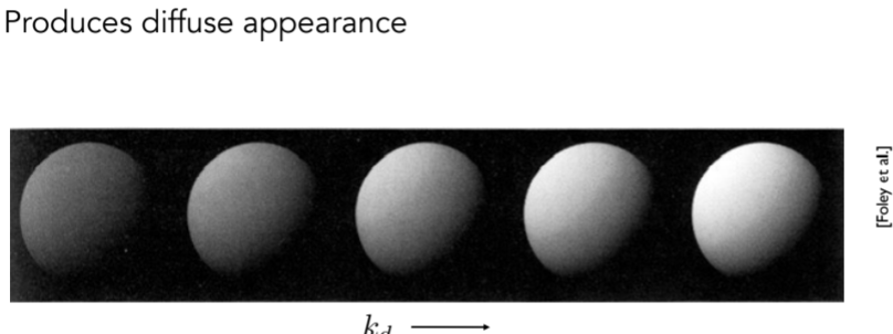
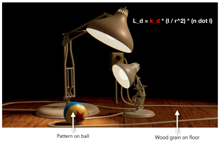
7.3.3.4. Lambertian (Diffuse) Shading:kd漫反射能量吸收系数,与视角向量无关
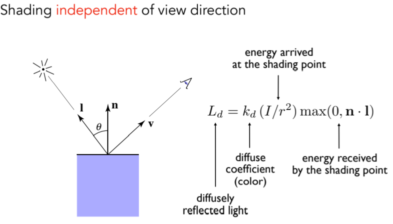
7.3.3.5. 问题:不考虑观测点到着色点的距离吗?
这个地方需要用到辐射亮度学的知识,先这样!!!
8. 第八讲-Shading 2 (Shading, Pipeline and Texture Mapping)
8.1. Blinn-Phong reflectance model
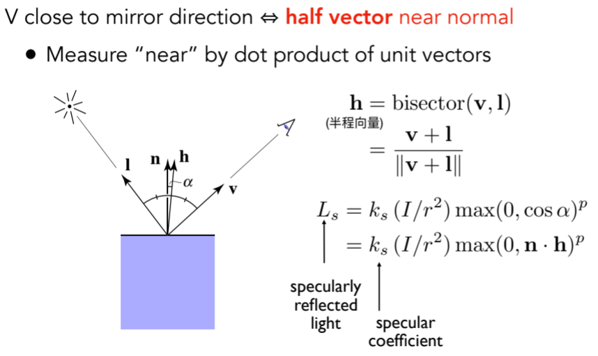
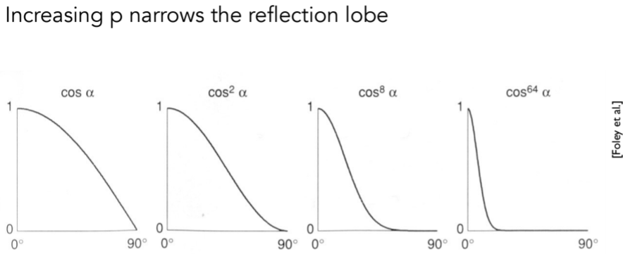
8.1.1. Specular
8.1.1.1. Intensity depends on view direction
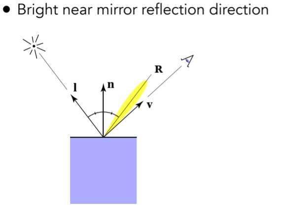
8.1.1.2. V和R之间的关系不便求解,因此提出用半程向量来衡量,同时类比漫反射的式子
8.1.1.3. 效果图

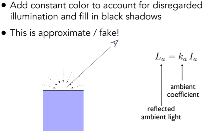
8.1.2. ambient terms
8.1.2.1. Shading that does not depend on anything,任一着色点接收环境光的相同的
8.1.3. 问题:磨砂材质是否完全没有高光?不一定,需要看磨砂的程度
8.2. Shading frequencies
8.2.1. What caused the shading difference?
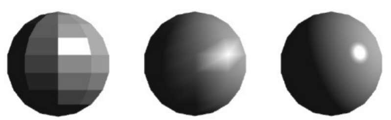
8.2.1.1. 左:Shade each triangle (flat shading)
对一个三角形或者四边形面片,用面法向着一个色

8.2.1.2. 中:Shade each vertex (Gouraud shading)
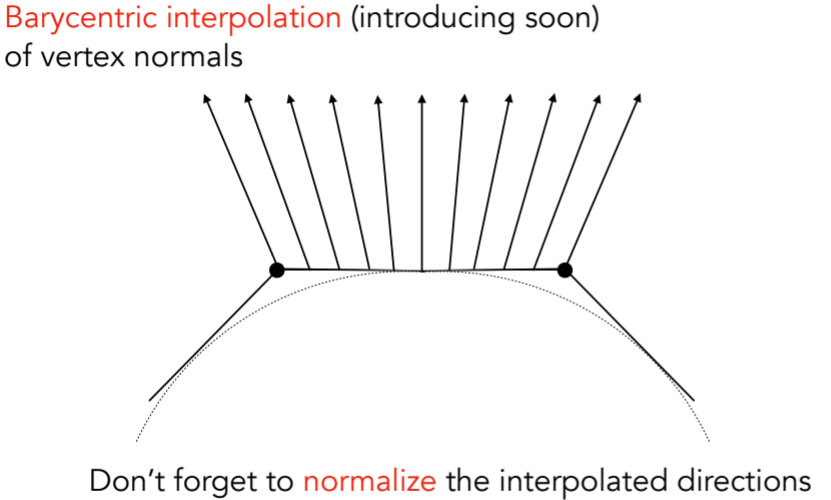
对面片的顶点法向着色,在三角形内部着色

8.2.1.3. 右:Shade each pixel (Phong shading)
每个像素着色,这里注意着色频率和着色模型的区别

8.2.2. Shading Frequency: Face, Vertex or Pixel:很难说那个更好,在面足够多时,也可以达到很好的着色效果

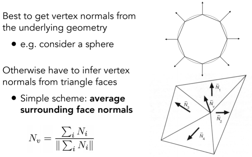
8.2.3. Defining Per-Vertex Normal Vectors(跟之前项目采样之后的操作很相似)
8.2.4. Defining Per-Pixel Normal Vectors
8.3. Graphics pipeline
8.3.1. Graphics Pipeline
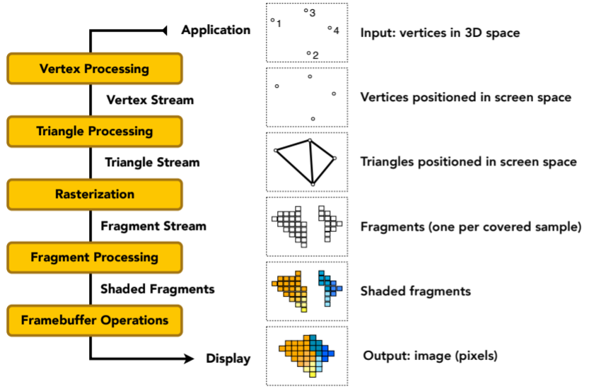
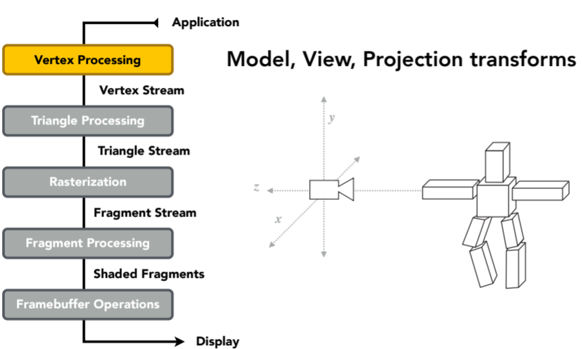
8.3.2. shading和texture maping这块最关键的是顶点着色(vertex shader,vertex processing阶段)还是像素着色(fragment shader,fragement processing阶段)
8.3.3. Shader Programs
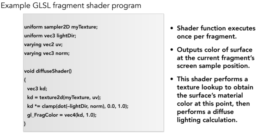

- Program vertex and fragment processing stages
- Describe operation on a single vertex (or fragment)
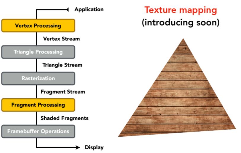
8.4. Texture Mapping纹理映射
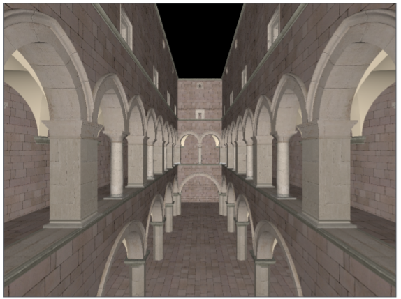
8.4.1. Different Colors at Different Places?观察球和地板,共用一套相同的反射模型,但是可以呈现不同的图案颜色,在物体不同位置定义不同属性,这就引出纹理映射
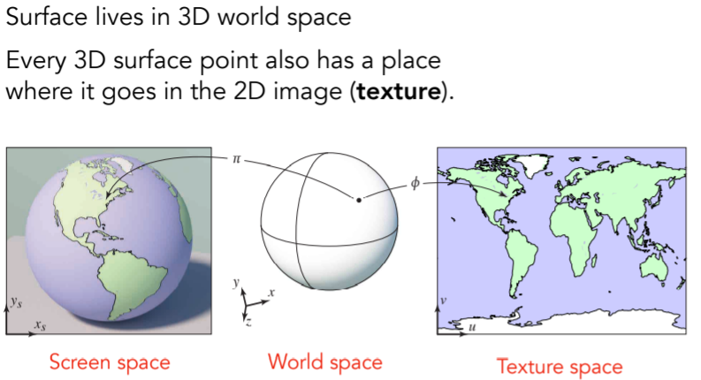
8.4.2. surfaces are 2D任意一个三维物体表面其实是二维的。定义在哪?定义在物体表面,简历表面和一张图的对应关系
8.4.2.1. Texture Applied to Surface

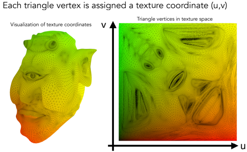
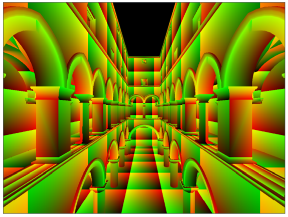
8.4.2.2. Visualization of Texture Coordinates
8.4.2.3. Texture Applied to Surface
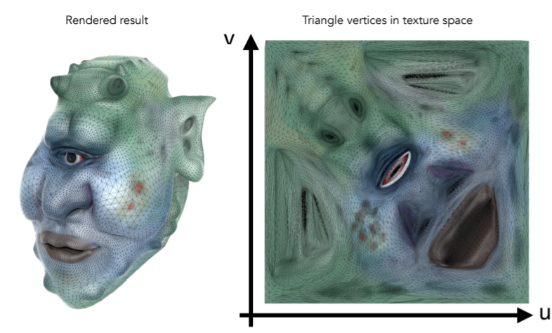
8.4.2.4. Textures applied to surfaces
8.4.2.5. Visualization of texture coordinates
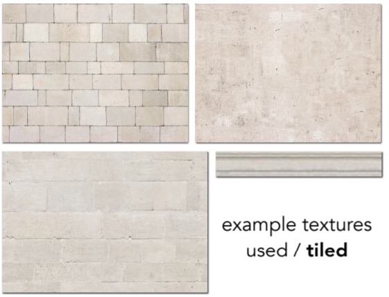
8.4.2.6. Textures can be used multiple times!
9. 第九讲-Shading 3 (Texture Mapping cont.)
9.1. Barycentric coordinates (Interpolation Across Triangles:)
9.1.1. Interpolation Across Triangles
9.1.1.1. Why do we want to interpolate?
    - Specify values at vertices
    - Obtain smoothly varying values across triangles
9.1.1.2. What do we want to interpolate?
- Texture coordinates, colors, normal vectors, …
9.1.1.3. How do we interpolate?
- Barycentric coordinates
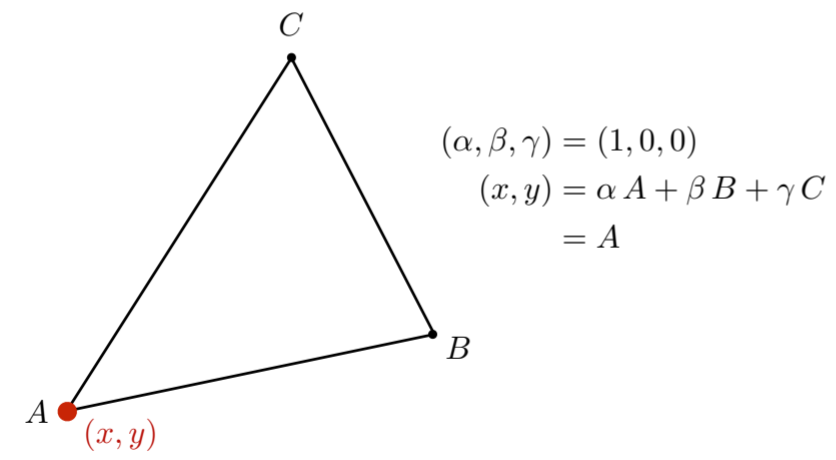
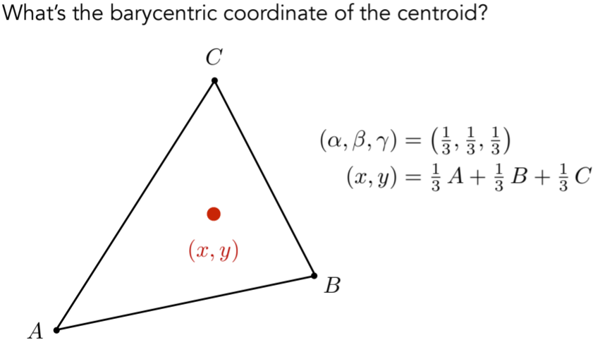
9.1.2. Barycentric Coordinates,这里的三个系数是重心坐标
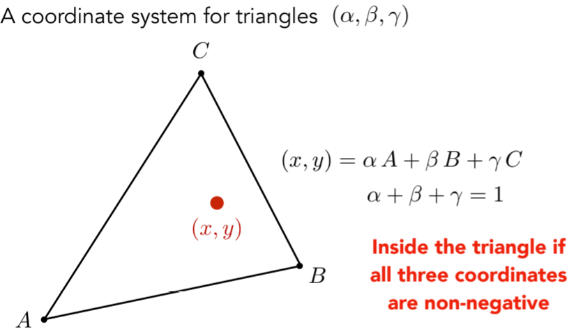
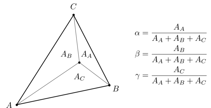
9.1.3. Geometric viewpoint — proportional areas用面积占比的方式计算重心坐标
9.1.4. Using Barycentric Coordinates

注意在投影变换下,三维空间下的重心坐标和投影之后的二维计算得到的重心坐标是不一样的,因此对于三维空间中的属性,需要先在三维中做插值,再投影到二维中去运用,这也就是重心坐标的局限性。
9.2. Texture queries
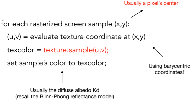
9.2.1. Simple Texture Mapping: Diffuse Color
9.2.2. texture中的问题:
9.2.2.1. Texture Magnification (What if the texture is too small?)
9.2.2.1.1. Texture Magnification - Easy Case纹理分辨率较低
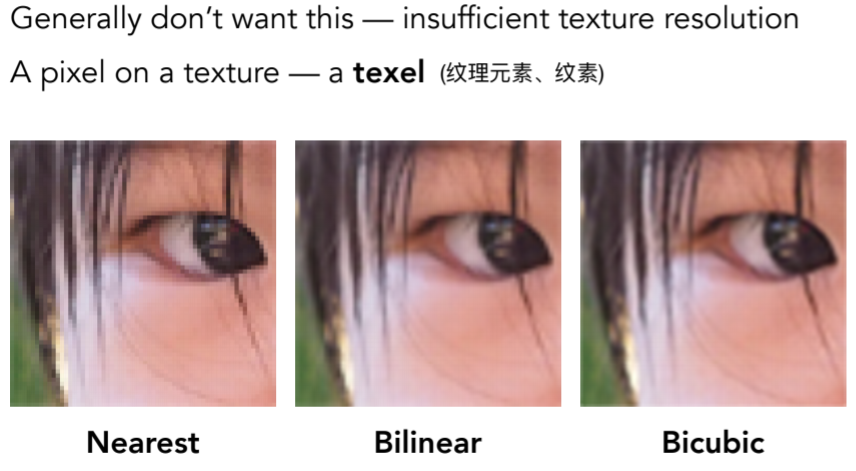
- nearest:此时 会映射到纹理的非整数位置,此时利用round算法映射为整数,即多个像素映射到同一个整型texel,锯齿状
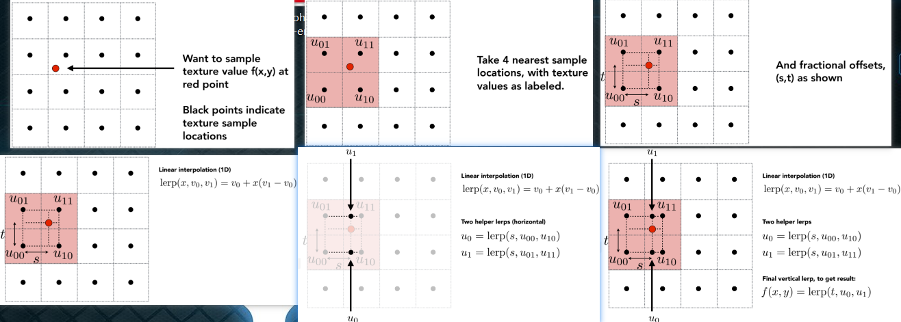
- 双线性插值Bilinear Interpolation:Bilinear interpolation usually gives pretty good results at reasonable costs
- bicubic插值
9.2.2.2. Texture Magnification (hard case) (What if the texture is too large?)
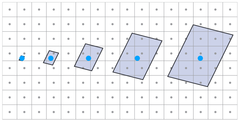
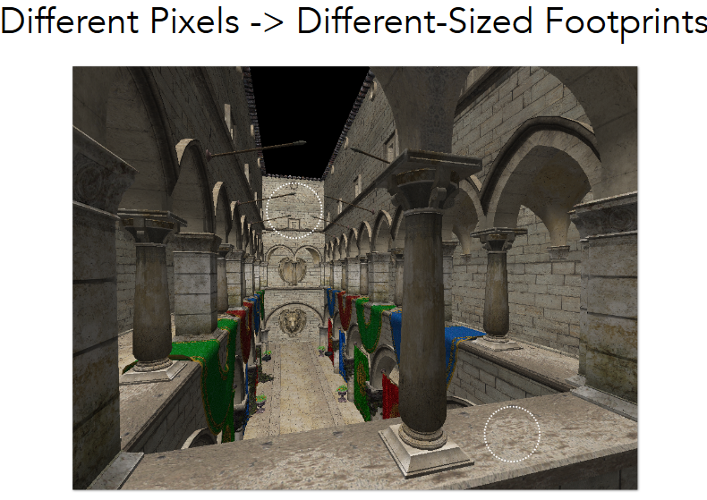
9.2.2.2.1. 会产生更为严重的问题,越远处,一个像素覆盖的纹素越多,也就是会
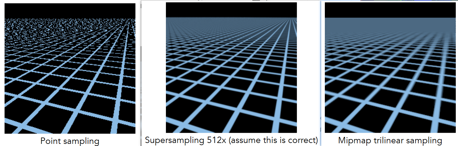
9.2.2.2.2. Point Sampling Textures — Problem
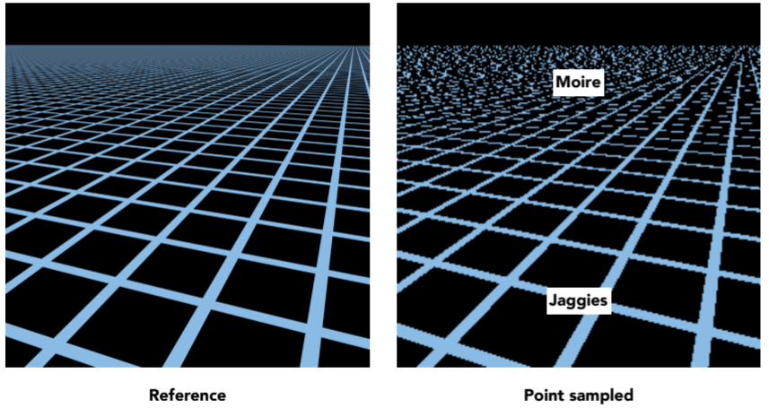
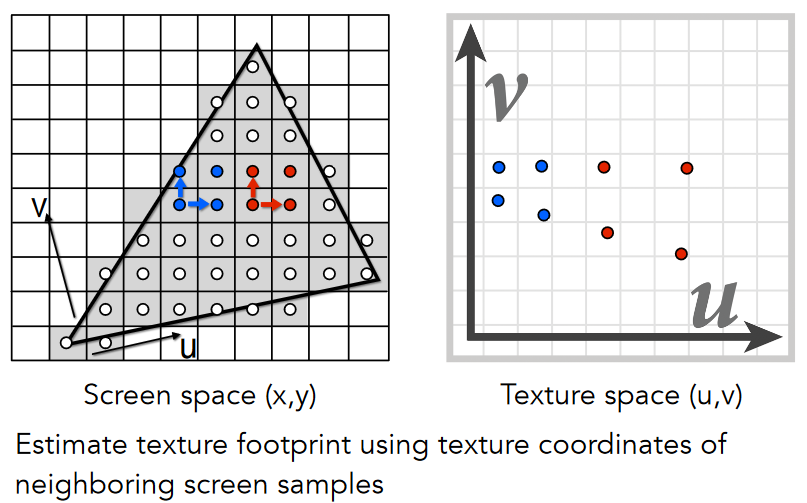
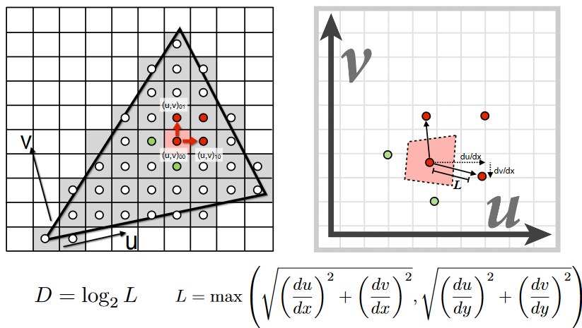
9.2.2.2.3. Screen Pixel “Footprint” in Texture

9.2.2.2.4. Will Supersampling Do Antialiasing?-最原始的想法 做supersample,但是这样耗费资源较大
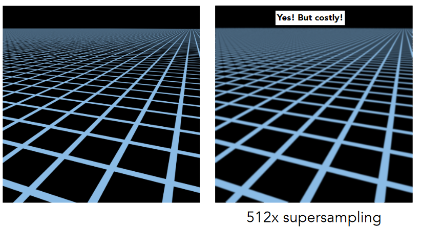
9.2.2.2.5. Antialiasing — Supersampling?

9.2.2.2.6. Point Query vs. (Avg.) Range Query构想:是否可以从前面的点查询转为范围查询
9.2.2.3. Mipmap - Allowing (fast, approx., square) range queries:估计值,因此是不准确的;只能做近似正方形的查询,在渲染之前把不同level的纹理都生成出来
9.2.2.3.1. Mipmap (L. Williams 83)
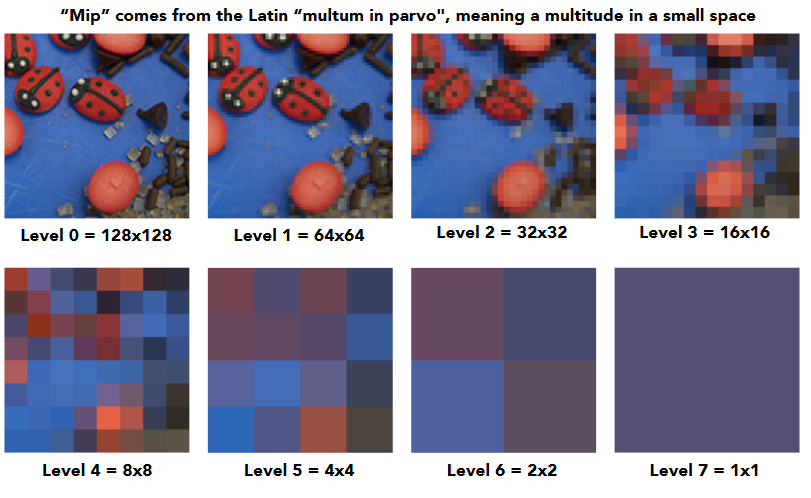
- What is the storage overhead of a mipmap?:根据上面的图可以看到,后一张纹理是前一张的四分之一,利用等比数列的公式可以计算得到 总存储量只多了三分之一
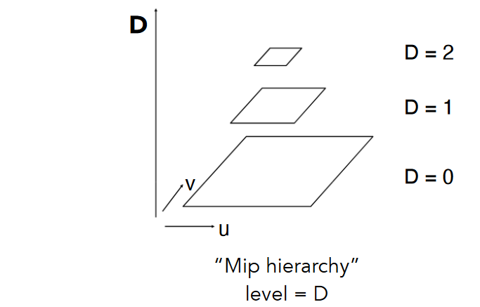
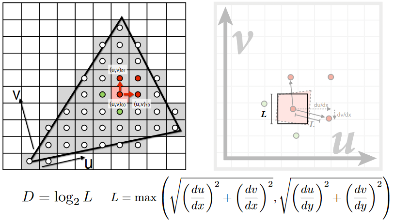
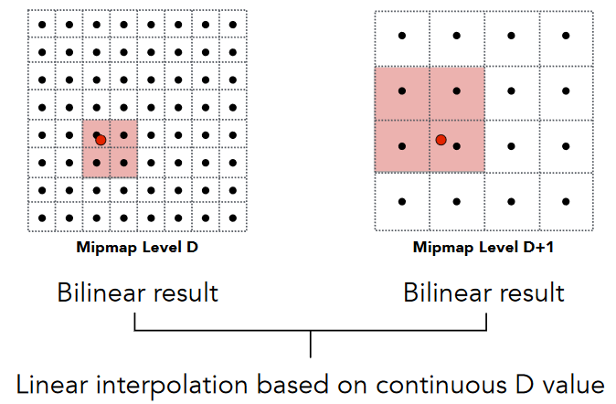
9.2.2.3.2. Computing Mipmap Level D
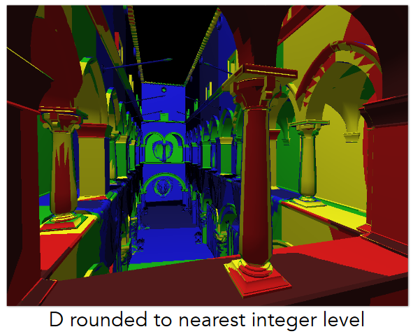
9.2.2.3.3. Visualization of Mipmap Level
9.2.2.3.4. Trilinear Interpolation
9.2.2.3.5. Visualization of Mipmap Level

9.2.2.3.6. Mipmap Limitations可以看到在最后的mipmap中,会出现很大的模糊,mipmap只能做正方块范围查询,做平均值,三线性插值也会不准
9.2.2.4. Anisotropic Filtering各向异性过滤
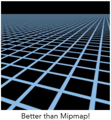
9.2.2.4.1. Irregular Pixel Footprint in Texture

9.2.2.4.2. Anisotropic Filtering

开销增加三倍,在不同方向上表现不同
9.3. Applications of textures
9.3.1. Many, Many Uses for Texturing
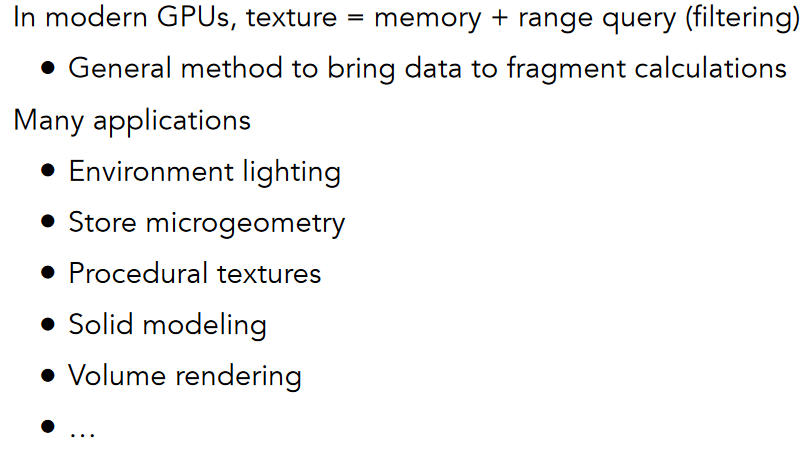
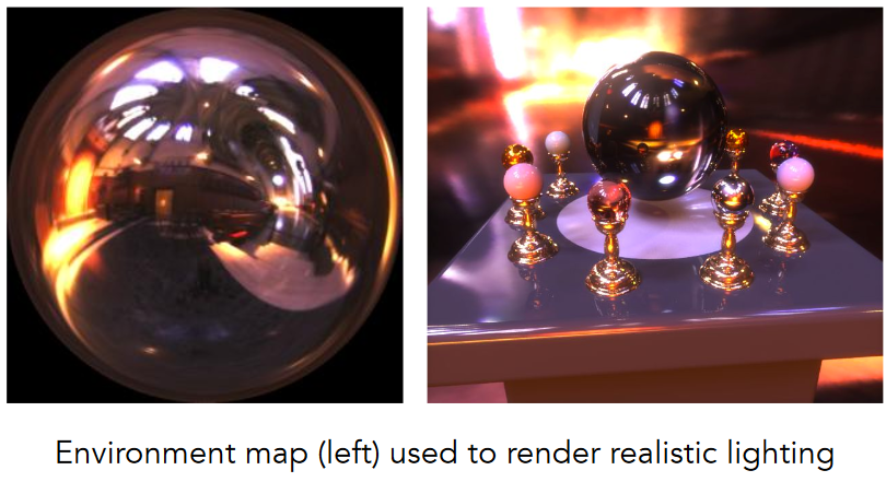
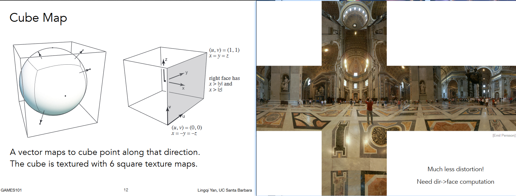
9.3.2. Environment Map用纹理描述环境图
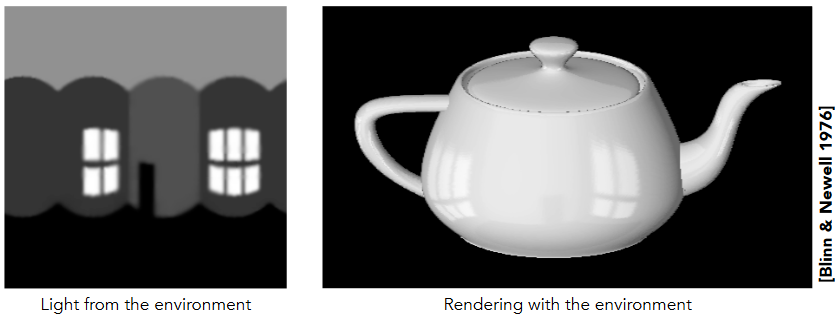
9.3.3. Environmental Lighting
9.3.4. Spherical Environment Map
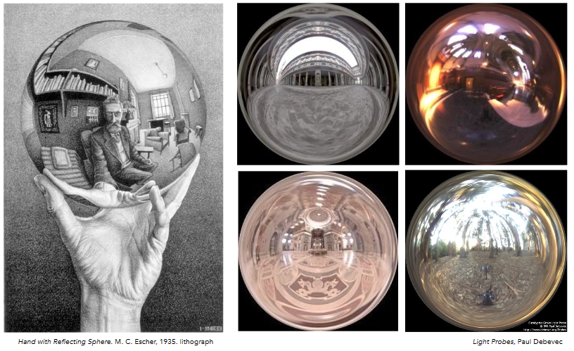
9.3.4.1. Spherical Map — Problem看最上面发现不是均匀的描述
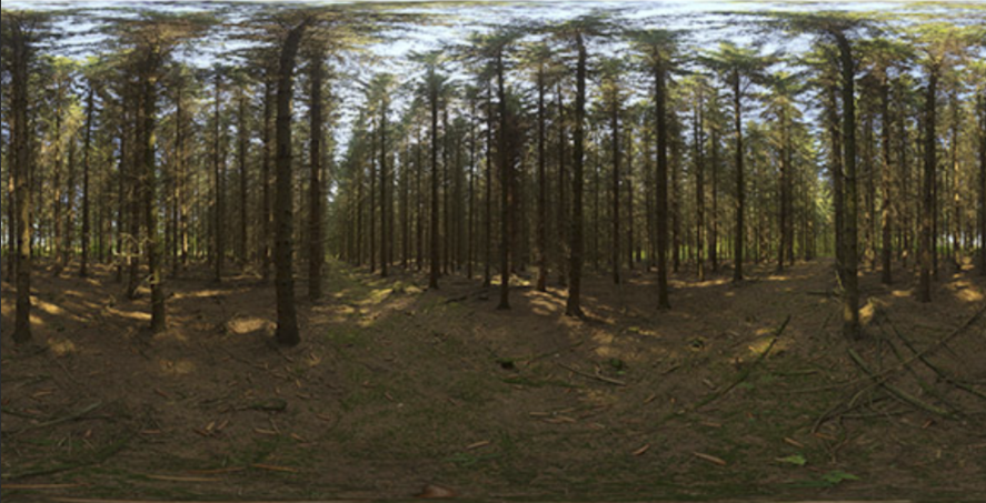
9.3.4.2. Cube Map从球壳上做球面投影到立方体上
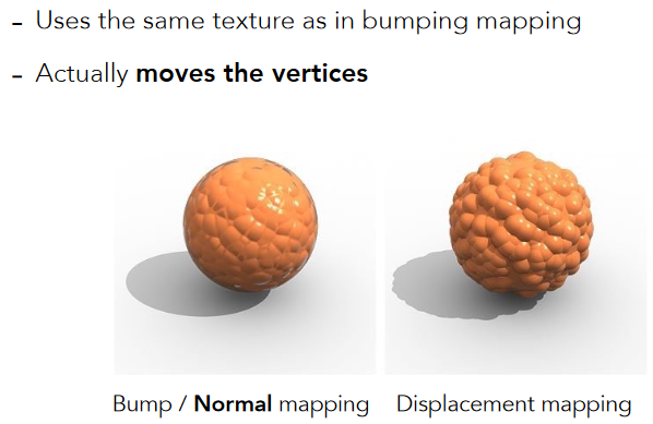
9.3.5. textures can affect shading凹凸贴图(法向贴图)
9.3.5.1. 并不一定代表颜色
- 
9.3.5.1.1. Bump Mapping
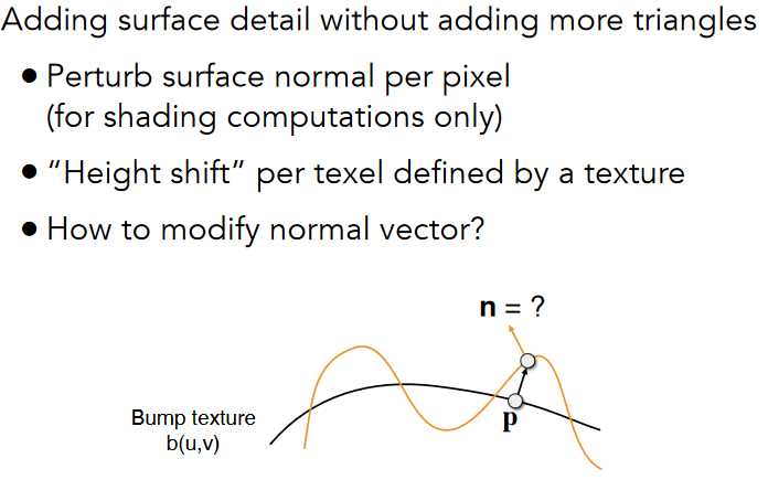
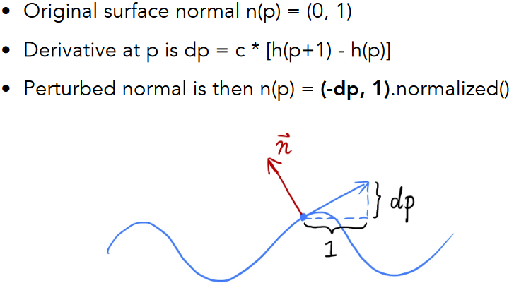
9.3.5.1.2. How to perturb the normal (in flatland)
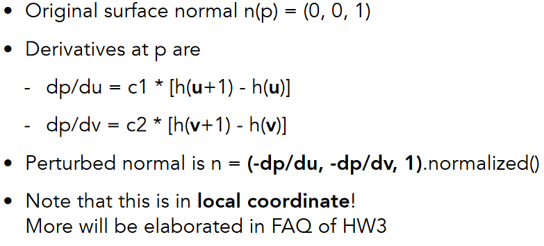
9.3.5.1.3. How to perturb the normal (in 3D)
9.3.5.2. Displacement mapping — a more advanced approach
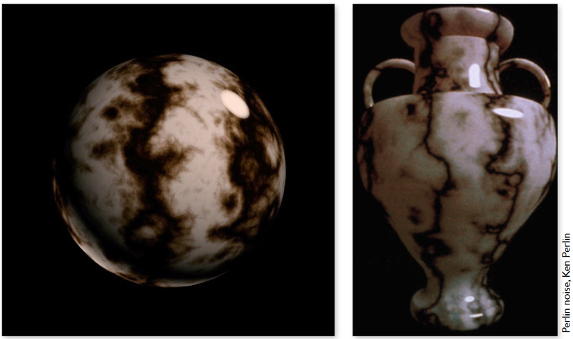
9.3.5.3. 3D Procedural Noise + Solid Modeling
9.3.5.4. Provide Precomputed Shading

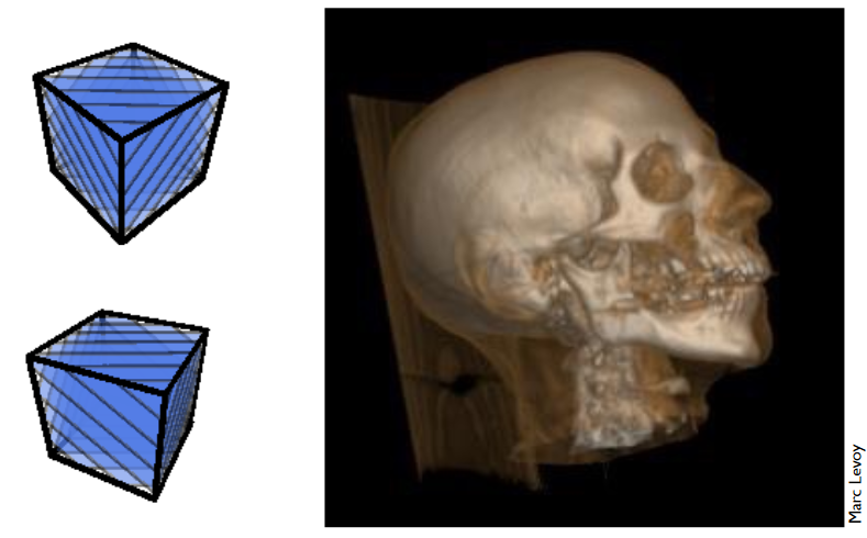
9.3.5.5. 3D Textures and Volume Rendering
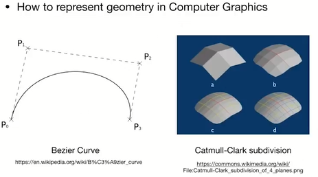
10. 第十讲-Geometry 1 - Introduction
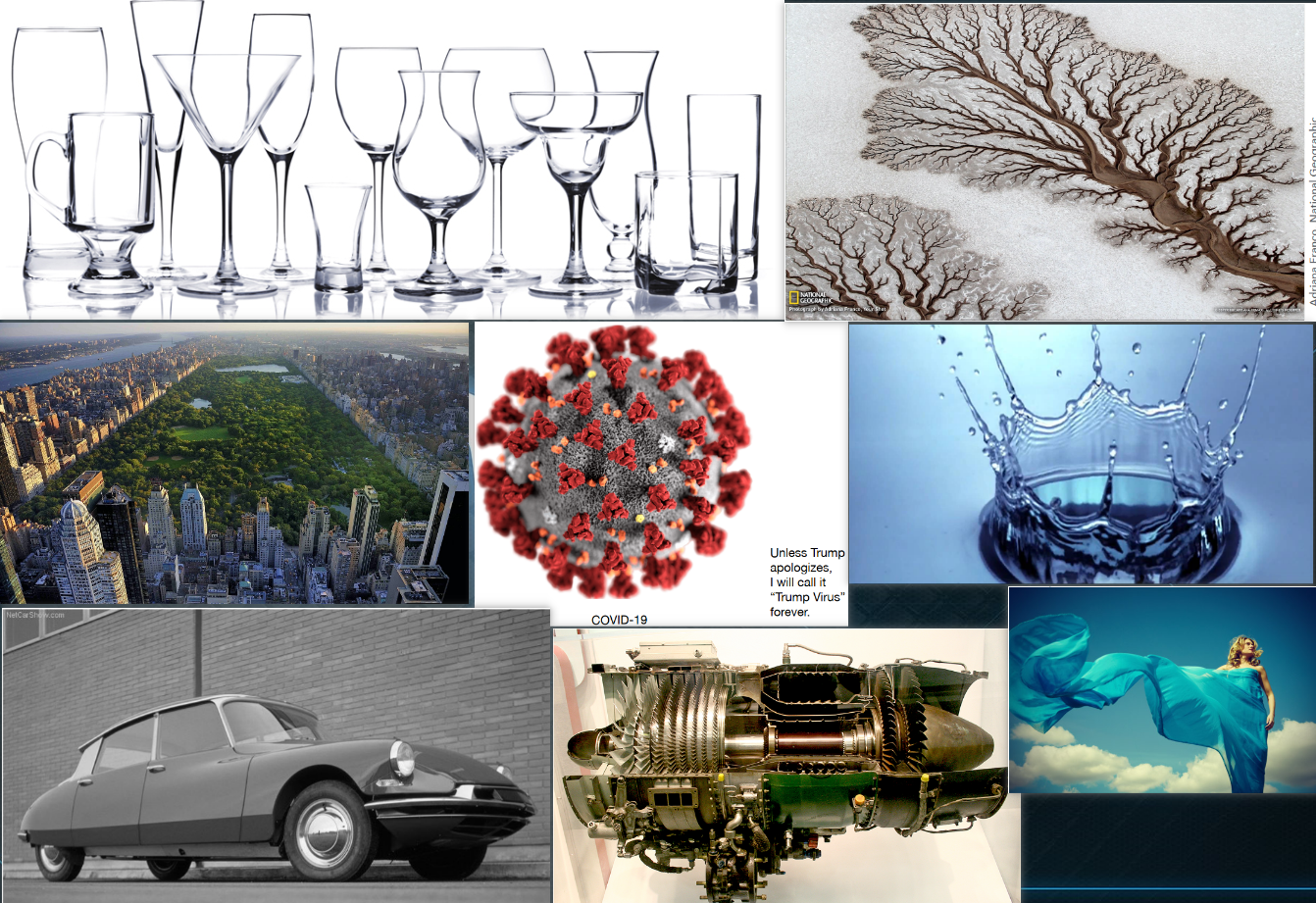
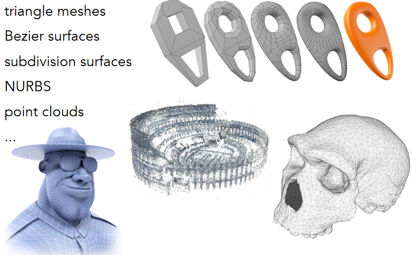
10.1. Examples of geometry
10.2. Various representations of geometry
10.2.1. 表达
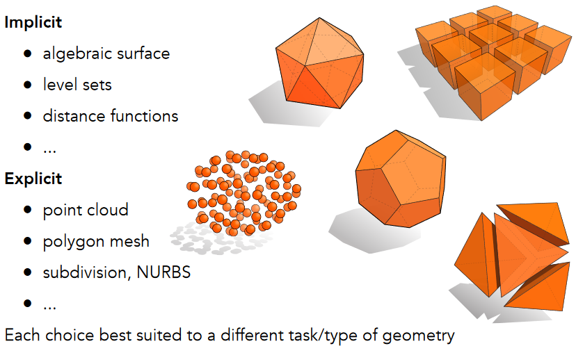
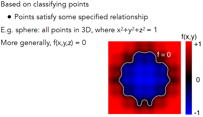
10.2.2. “Implicit” Representations of Geometry
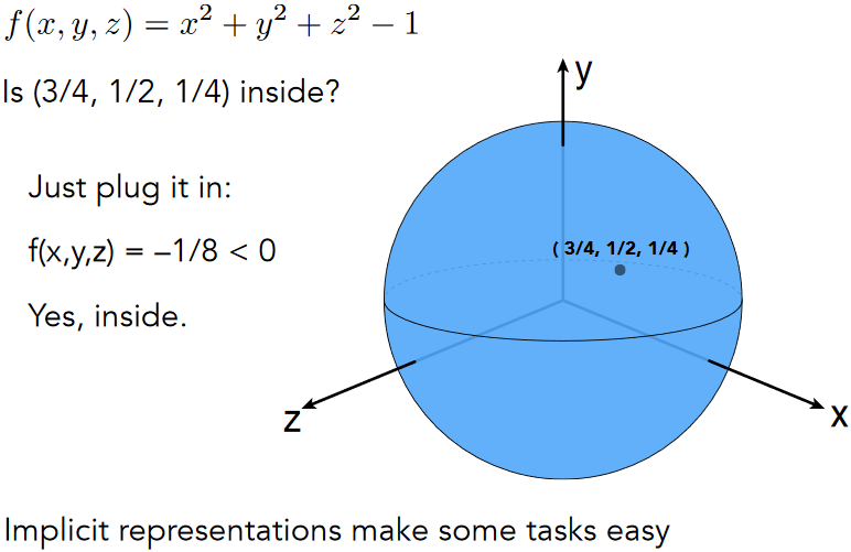
10.2.2.1. 不告诉具体的位置 只告诉满足的某种关系,很难去找到所有的点的具体 位置,但是可以很方便的判断点是否在在surface内外
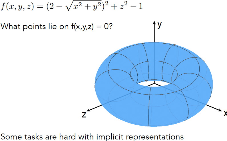
10.2.2.2. Implicit Surface – Sampling Can Be Hard
10.2.2.3. Implicit Surface – Inside/Outside Tests Easy
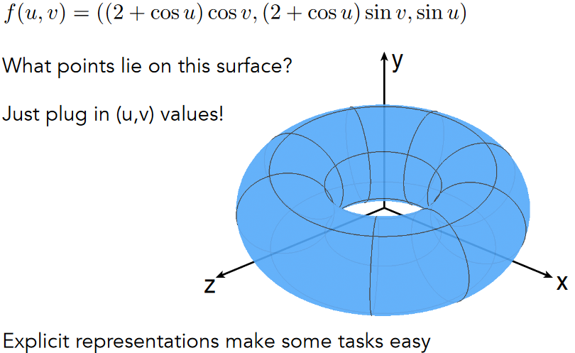
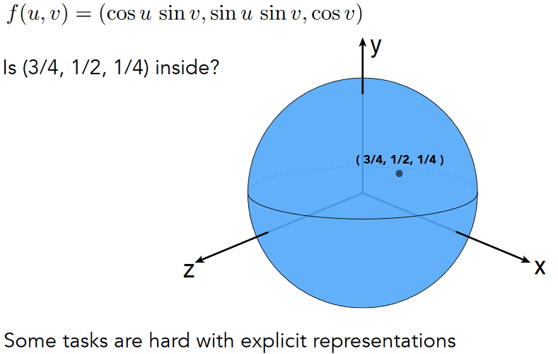
10.2.3. “Explicit” Representations of Geometry
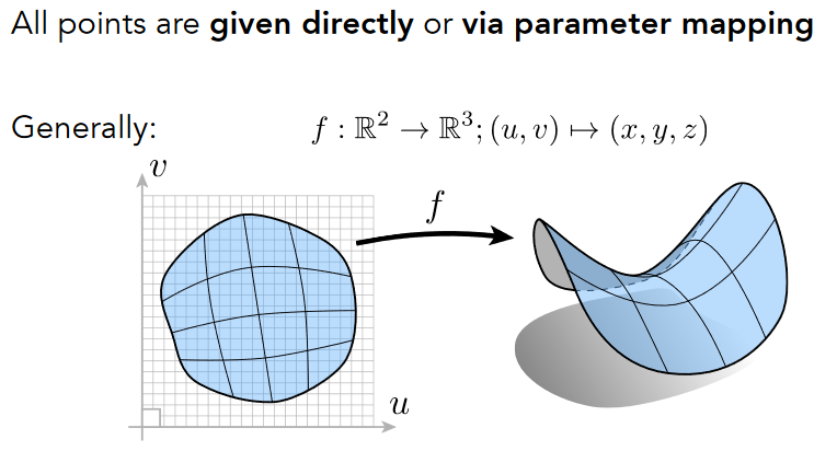
10.2.3.1. Explicit Surface – Sampling Is Easy
10.2.3.2. Explicit Surface – Inside/Outside Test Hard
10.2.4. No “Best” Representation – Geometry is Hard!根据需要选择合适的表达方式
10.2.5. More Implicit Representations in Computer Graphics
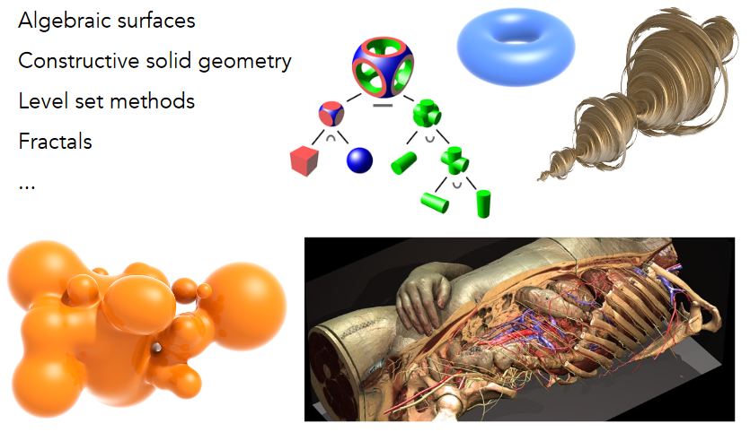
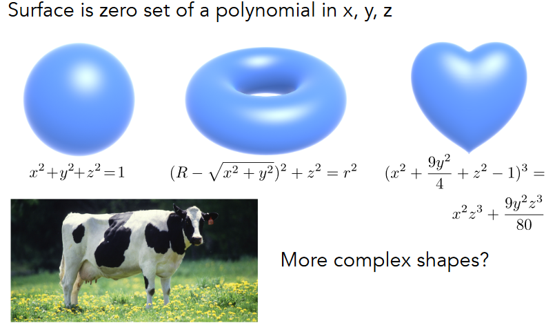
10.2.5.1. Algebraic Surfaces (Implicit)
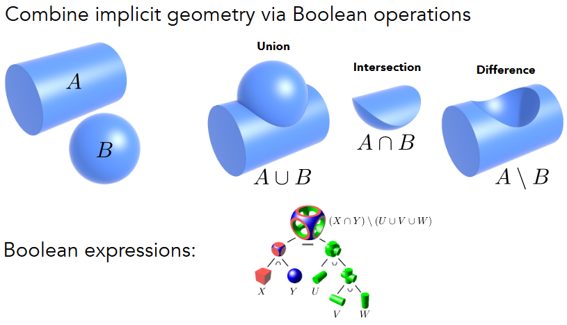
10.2.5.2. Constructive Solid Geometry (Implicit) - CSG
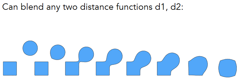
10.2.5.3. Distance Functions (Implicit)
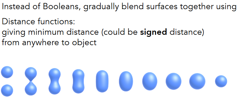

如果直接对图形blend,会发现如第一行的第三个结果 黑灰中,若想得到黑白一半的情况,则需要用有向距离函数
10.2.5.4. Blending Distance Functions (Implicit)
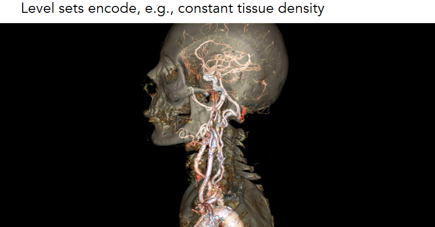
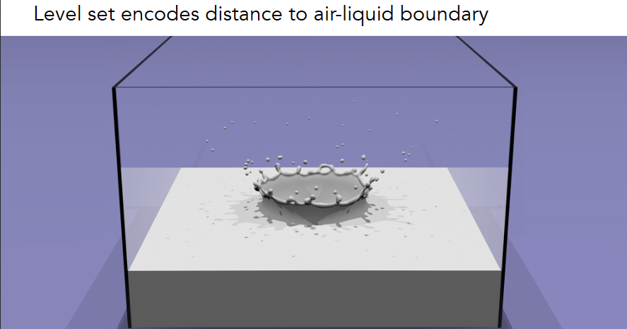
10.2.5.5. Level Set Methods (Also implicit)水平集,注意与distance function的差别

10.2.5.5.1. Level Sets from Medical Data (CT, MRI, etc.)
10.2.5.5.2. Level Sets in Physical Simulation
10.2.5.6. Fractals (Implicit)
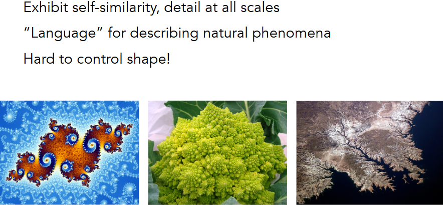
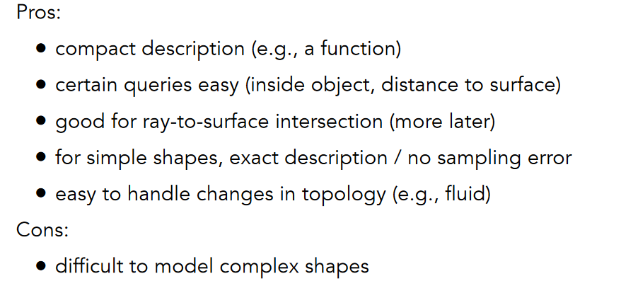
10.2.5.7. Implicit Representations - Pros & Cons
11. Lecture 11 Geometry 2 (Curves and Surfaces)
11.1. Explicit Representations
11.1.1. Many Explicit Representations in Graphics
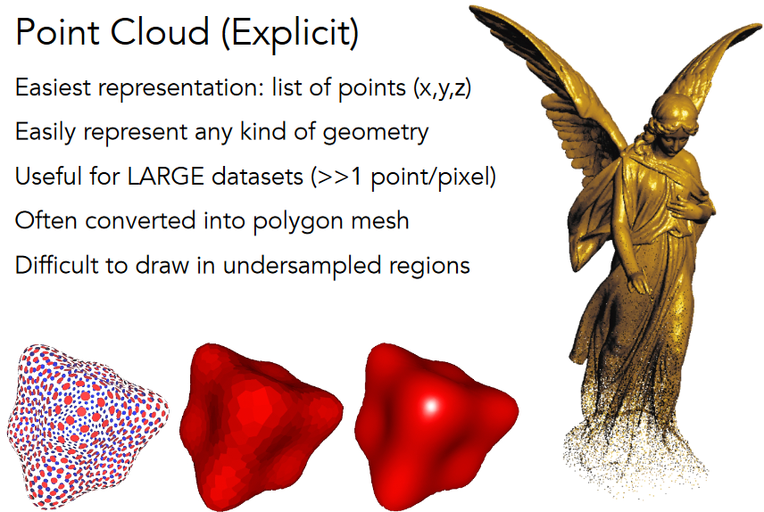
11.1.2. Point Cloud (Explicit)
11.1.3. Polygon Mesh (Explicit)

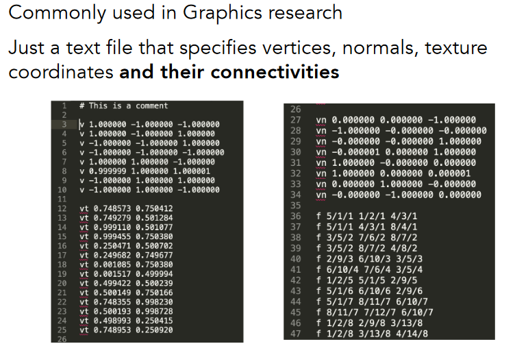
11.1.4. The Wavefront Object File (.obj) Format
11.2. Curves

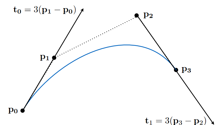
11.2.1. -Bezier curves 贝塞尔曲线
11.2.1.1. Defining Cubic Bézier Curve With Tangents:1.起点和终点;2.起始方向必须过p0p1,终止方向必须过p2p3看,其他的控制点则不强制性通过
11.2.1.2. Evaluating Bézier Curves -De Casteljau’s algorithm :动态展示http://acko.net/
11.2.1.2.1. Bézier Curves – de Casteljau Algorithm:把所有t时间的点都画出来 连起来就是贝塞尔曲线

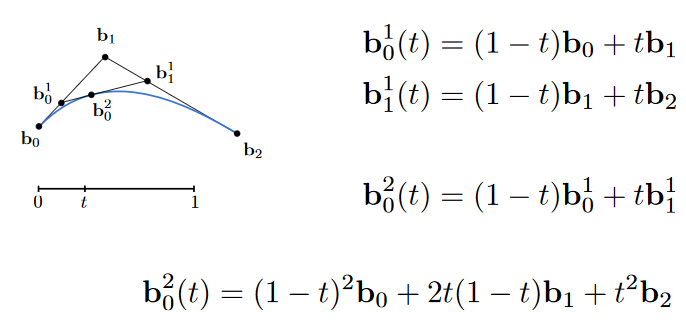
11.2.1.3. Evaluating Bézier Curves - Algebraic Formula
11.2.1.3.1. de Casteljau algorithm gives a pyramid of coefficients

11.2.1.3.2. Example: quadratic Bézier curve from three points
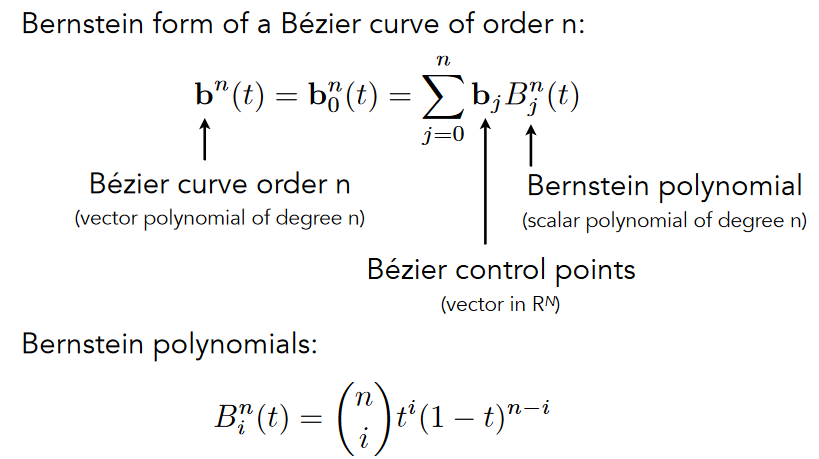
11.2.1.3.3. Bézier Curve – General Algebraic Formula
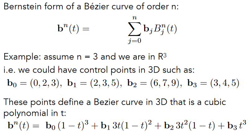
11.2.1.3.4. Bézier Curve – Algebraic Formula: Example
11.2.1.3.5. Cubic Bézier Basis Functions
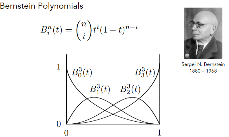
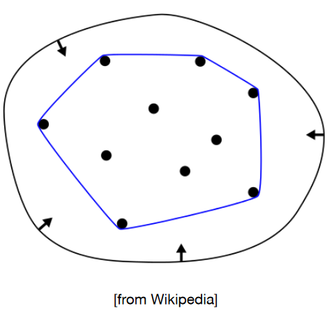
11.2.1.3.6. Properties of Bézier Curves
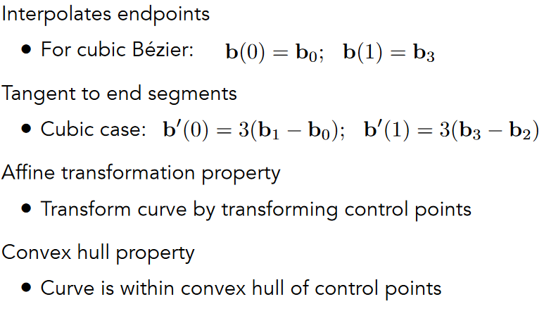
- BTW: What’s a Convex Hull
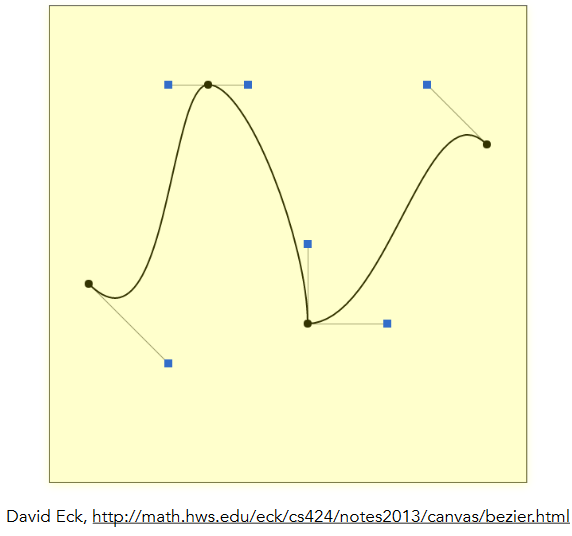
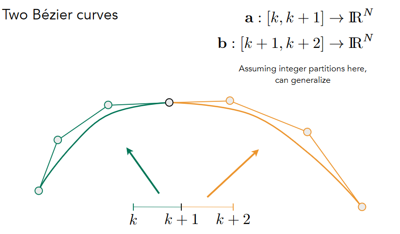
11.2.1.4. Piecewise Bézier Curves
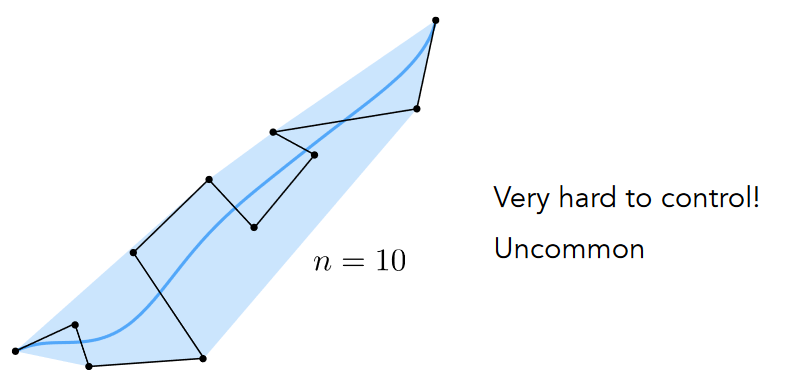
11.2.1.4.1. Higher-Order Bézier Curves?
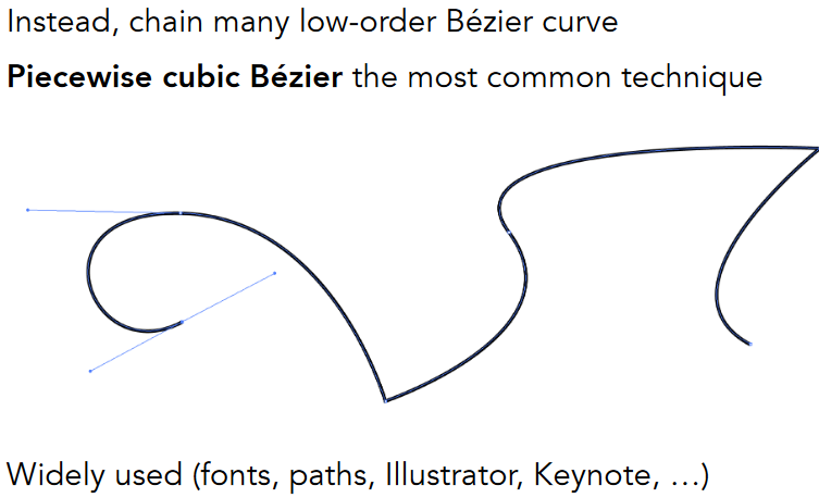
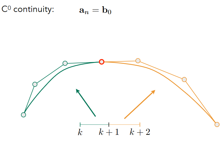
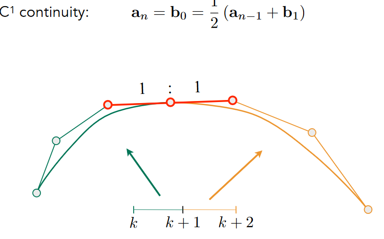
11.2.1.4.2. Demo – Piecewise Cubic Bézier Curve:两段曲线之间用终止和起始向量一致来控制,长度一样 方向相反
11.2.1.4.3. Continuity
11.2.2. Other types of splines
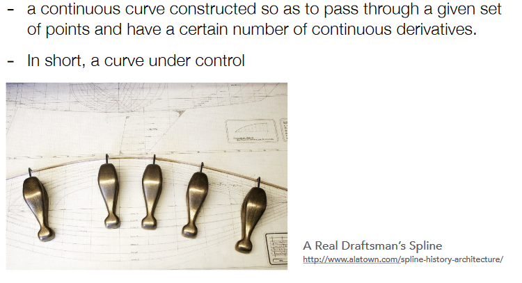
11.2.2.1. Spline样条
11.2.2.2. B-splines, etc.
11.3. Surfaces
11.3.1. -Bezier surfaces
11.3.1.1. Extend Bézier curves to surfaces
11.3.1.2. Bicubic Bézier Surface Patch

11.3.1.3. Visualizing Bicubic Bézier Surface Patch http://acko.net
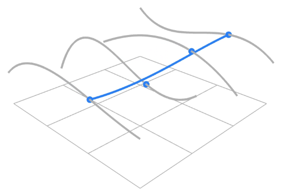
11.3.1.4. Evaluating Bézier Surfaces
11.3.1.4.1. Evaluating Surface Position For Parameters (u,v)

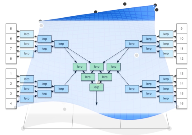
11.3.1.4.2. Method: Separable 1D de Casteljau Algorithm
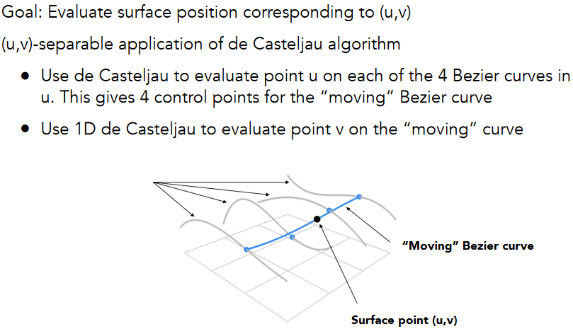
11.3.1.4.3. Method: Separable 1D de Casteljau Algorithm
11.3.2. -Triangles & quads
11.3.2.1. -Subdivision, simplification, regularization

12. Lecture 12:Geometry 3
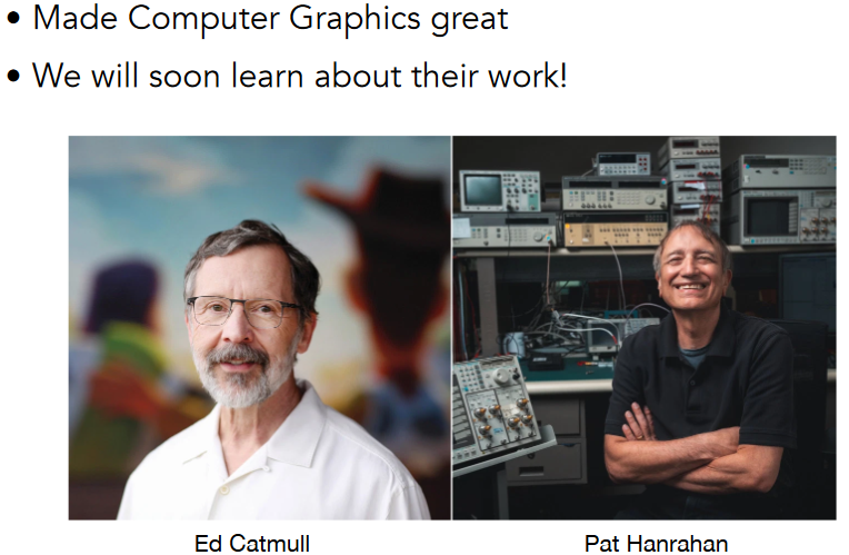
12.1. Turing Award Winners
12.2. Mesh Operations: Geometry Processing
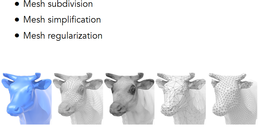
12.2.1. Mesh Subdivision (upsampling)

12.2.1.1. Loop subdivision(Loop :family name,不是循环)
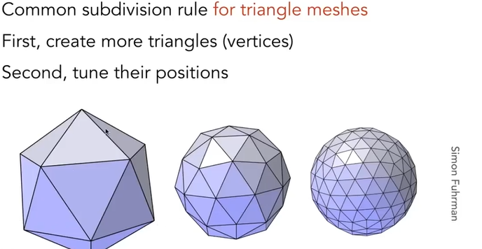
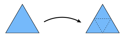
12.2.1.1.1. first:Split each triangle into four
12.2.1.1.2. second:Assign new vertex positions according to weights ,New / old vertices updated differently

      - Loop Subdivision — Update

        - new vertices,以其中的一个新生成的白点为例
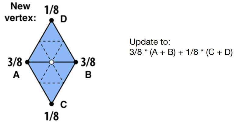
- old vertices (e.g. degree 6 vertices here):degree即为某个点连了几条边,度越高,直观的理解就是多参考邻域的信息

12.2.1.1.3. Loop Subdivision Results

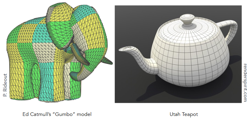
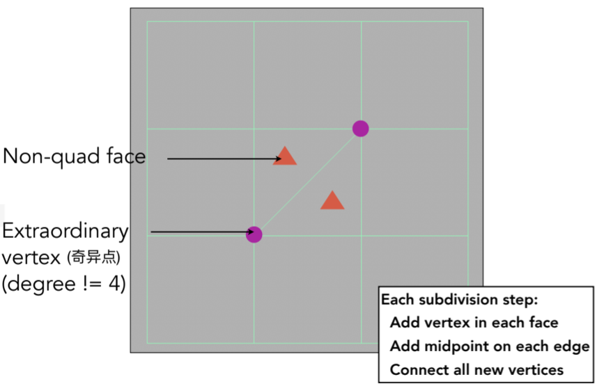
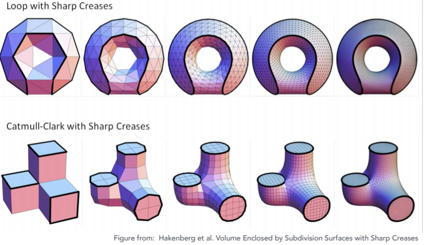
12.2.1.2. Catmull-Clark Subdivision (General Mesh)
12.2.1.2.1. why?
因为Loop subdivision只能用于三角形的面片,因此需要提出一个更一般的情况
12.2.1.2.2. 一些基本的定义
quad face四边形面 Non-quad face非四边形面;奇异点:只要是度不等于4的点;每一次分解先在每一个面添加一个点,再在边上添加一个点,最后连接新的点。在每一个subdivision之后,每一个非四边形面新增两个奇异点,非四边形面消失

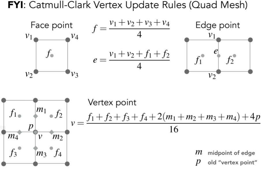
12.2.1.2.3. 顶点更新规则
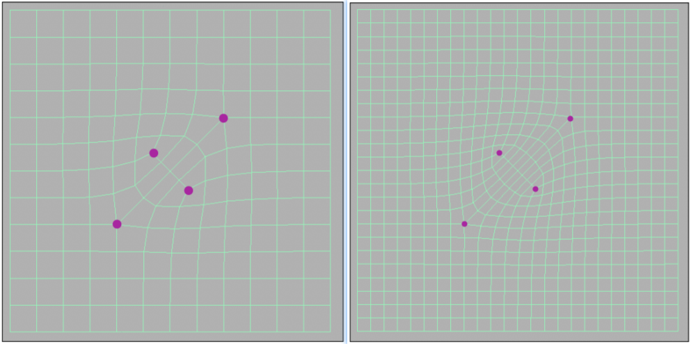
12.2.1.2.4. Convergence: Overall Shape and Creases
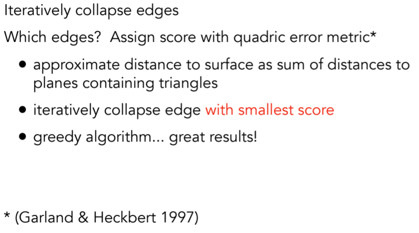
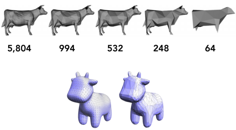
12.2.2. Mesh Simplification (downsampling):reduce number of mesh elements while maintaining the overall shape
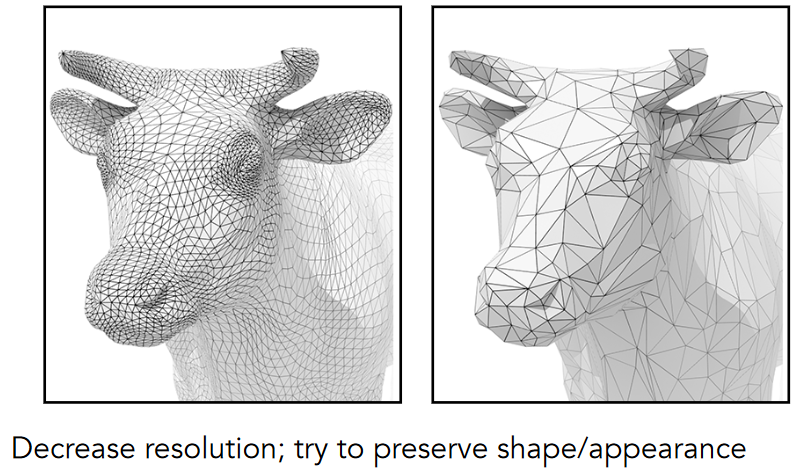
12.2.2.1. how?
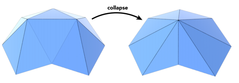
12.2.2.1.1. collapsing An edge边坍缩
- Suppose we simplify a mesh using edge collapsing
- 引入一个概念:Quadric Error Metrics(二次误差度量)
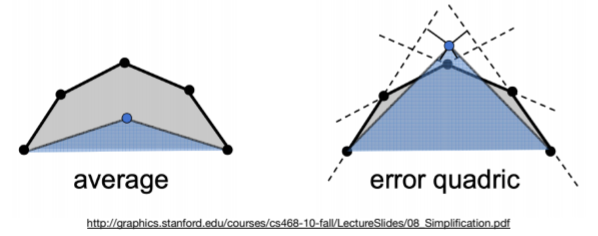
        - • How much geometric error is introduced by simplification?
        - • Not a good idea to perform local averaging of vertices (上图左):这种情况下新简化的三角形(蓝色表示)无法表征原始面片(灰色表示)
        - Quadric error: new vertex should minimize its sum of square distance (L2 distance) to previously related triangle planes!(上图右)

      - Quadric Error of Edge Collapse
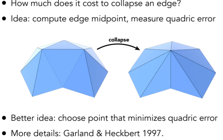
- Simplification via Quadric Error
- result:对于平的地方 坍缩会多一点
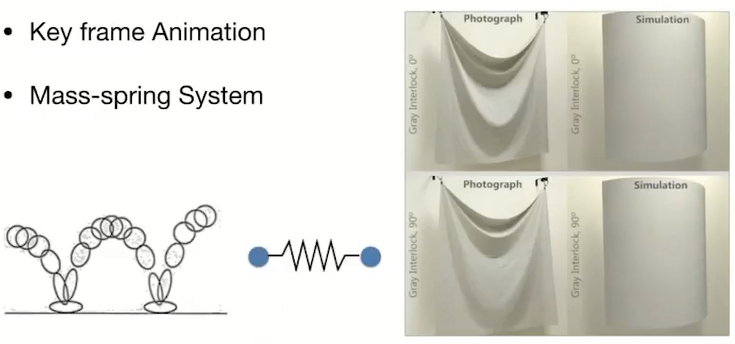
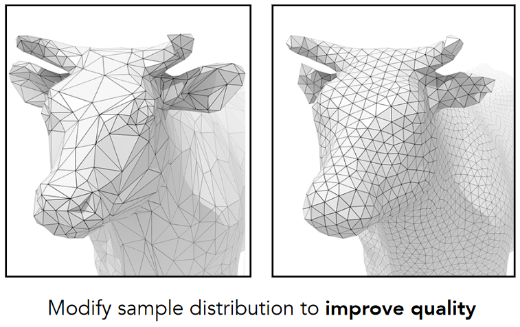
12.2.3. Mesh Regularization (same #triangles)大小三角形更均匀一些
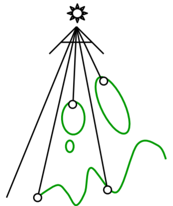
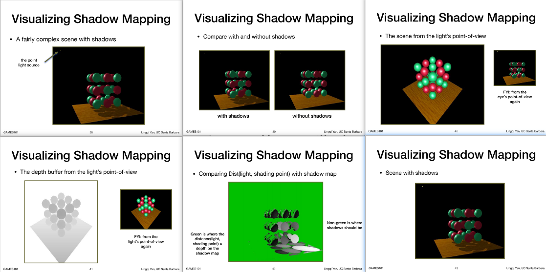
12.3. Shadow Mapping
12.3.1. an image-space algorithm
12.3.1.1. no knowledge of scene’s geometry during shadow computation在做shadow mapping的时候不需要知道场景几何信息
12.3.1.2. must deal with aliasing artifacts会产生走样现象
12.3.2. key idea:the points NOT in shadow must be seen both by the light and by the camera
12.3.3. 操作步骤:
12.3.3.1. pass 1:Render from Light
- Depth image from light source 从光源看场景,得到所看到点的深度图
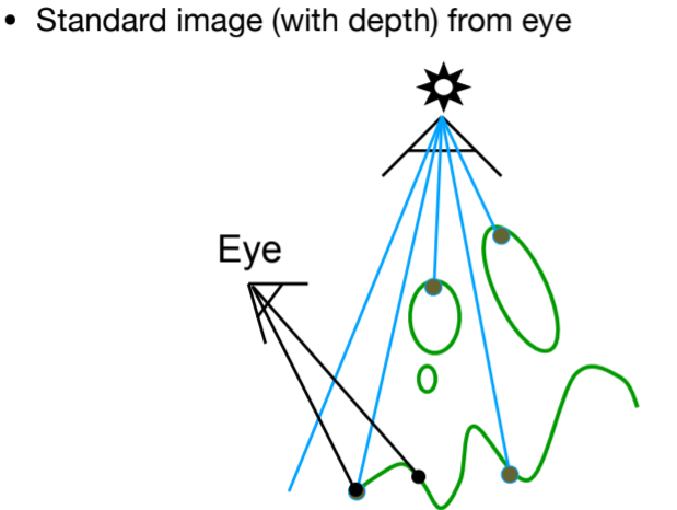
12.3.3.2. pass 2a:Render from Eye
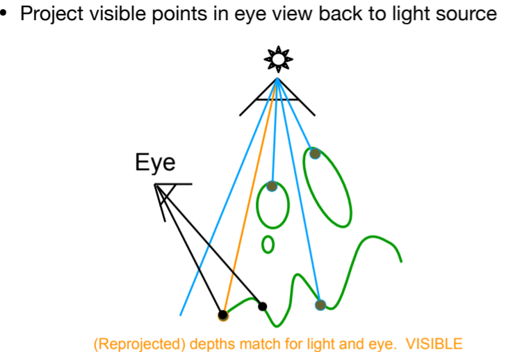
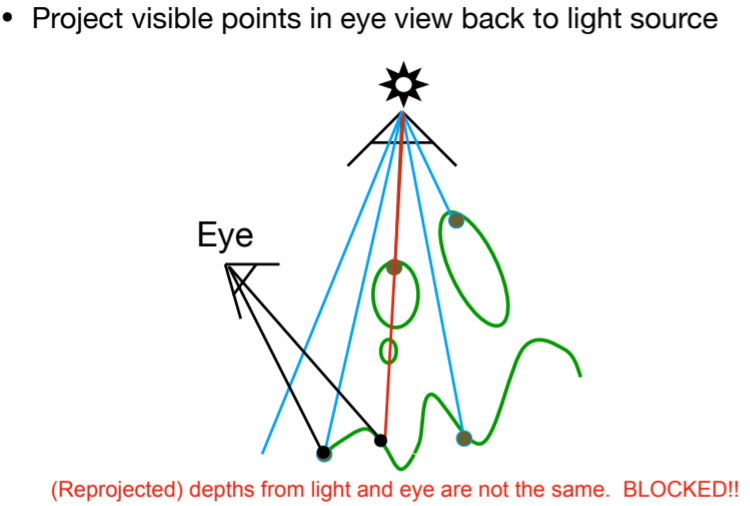
12.3.3.3. Pass 2B: Project to light
12.3.4. 可视化
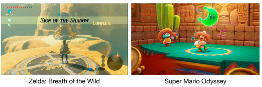
12.3.5. 很多知名的渲染技术用的就是shadow mapping
12.3.6. Basic shadowing technique for early animations (Toy Story, etc.) and in EVERY 3D video game
12.3.7. Problems with shadow maps
12.3.7.1. Hard shadows (point lights only) ,软阴影看起来就比较自然些。硬阴影,即为那些完全看不到光的,软阴影为那些部分可见的。后续有人也做了软阴影
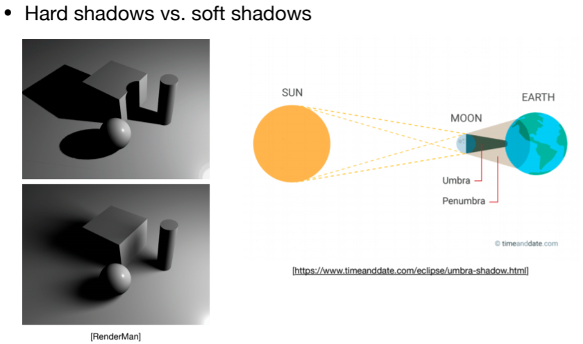
Quality depends on shadow map resolution (general problem with image-based techniques)
Involves equality comparison of floating point depth values means issues of scale, bias, tolerance
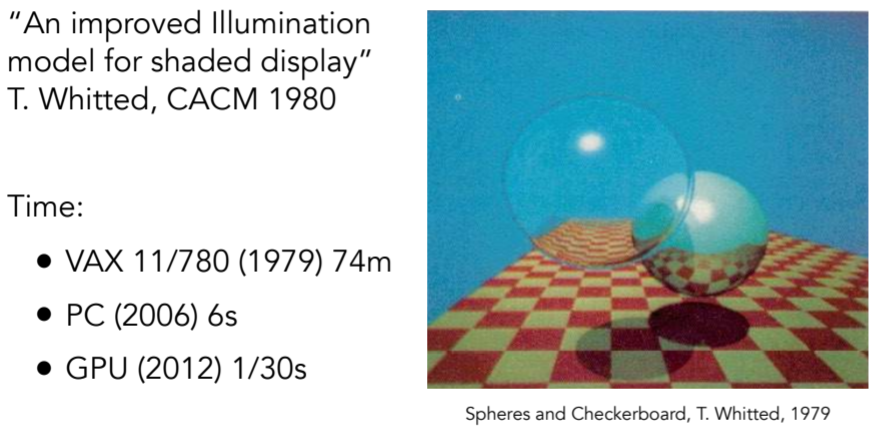
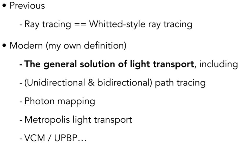
13. Lecture 13: Ray Tracing 1 (Whitted-Style Ray Tracing)
13.1. Why Ray Tracing?
13.1.1. Rasterization couldn’t handle global effects well
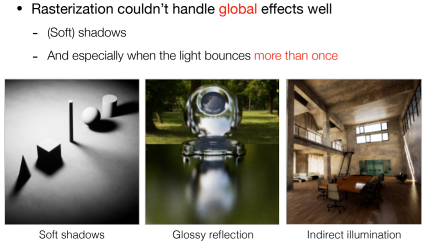
13.1.2. Rasterization is fast, but quality is relatively low
13.1.3. Ray tracing is accurate, but is very slow
13.2. Basic Ray-Tracing Algorithm
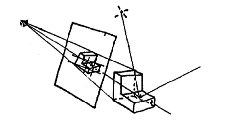
13.2.1. Light Rays(Three ideas about light rays)
- Light travels in straight lines (though this is wrong)
- Light rays do not “collide” with each other if they cross (though this is still wrong)
- Light rays travel from the light sources to the eye (but the physics is invariant under path reversal - reciprocity可逆性).
13.2.2. Ray Casting,简单的光线投射模型,还是认为光源只反射一次
13.2.2.1. Appel 1968 - Ray casting
    - \1. Generate an image by casting one ray per pixel ,首先从视角或者相机对屏幕的每个像素发出一条光线
    - \2. Check for shadows by sending a ray to the light 根据第一步得到的点在连接光源,看该点是否在阴影内,若不在又能被视角看到 则投射到屏幕上
13.2.2.2. Ray Casting - Generating Eye Rays
这里注意从eye point投射的光线跟场景的交点,只关注最近的相交点
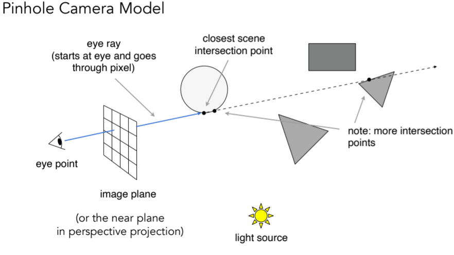
13.2.2.3. Ray Casting - Shading Pixels (Local Only)
从相交点连接光源,判断是否光源可见,若不在阴影内,则计算局部shading得到像素颜色

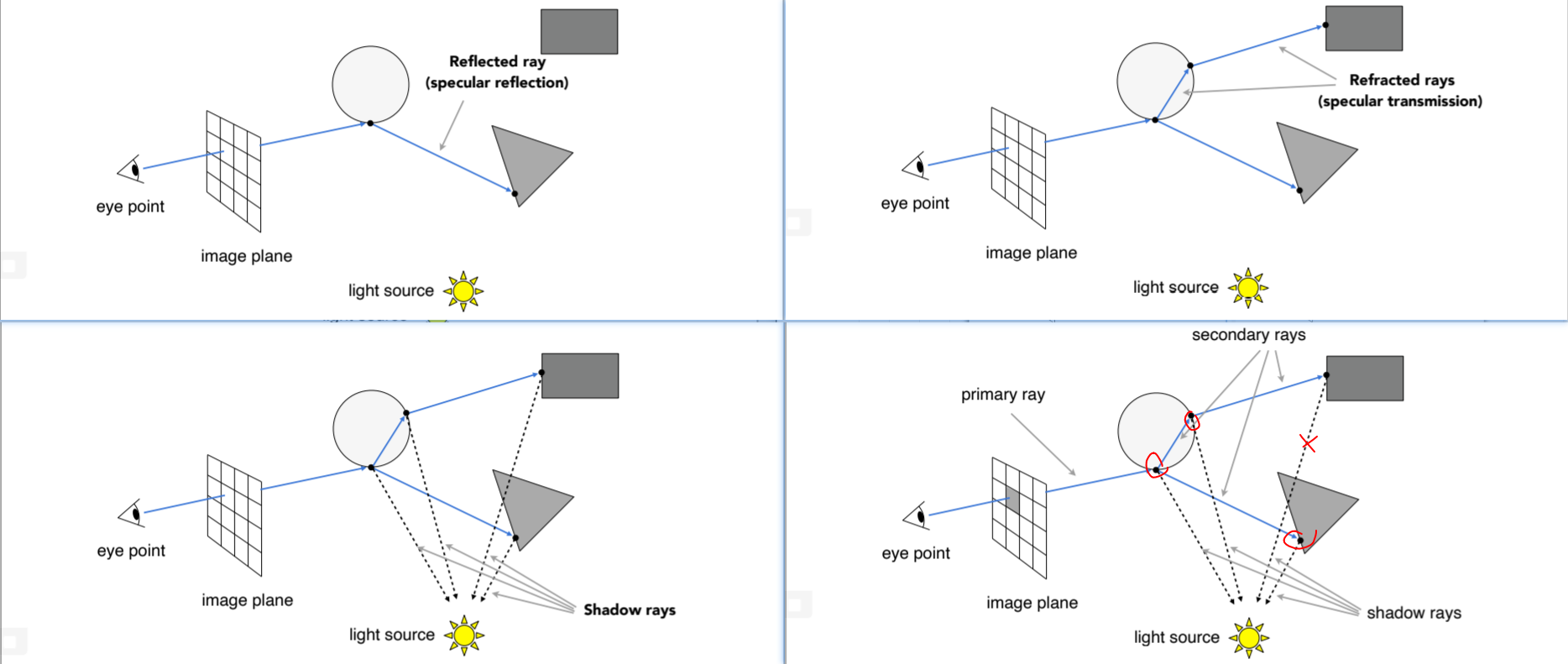
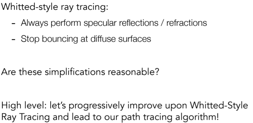
13.2.3. Recursive (Whitted-Style) Ray Tracing递归,完美反射和折射,多次计算光线传播方向
13.2.3.1. introduction
13.2.3.2. Recursive Ray Tracing ,注意这里的反射和折射,在昨晚shadow rays判断之后 会把可见的着色(红圈处)都加到pixel上面
13.2.3.3. 技术问题:
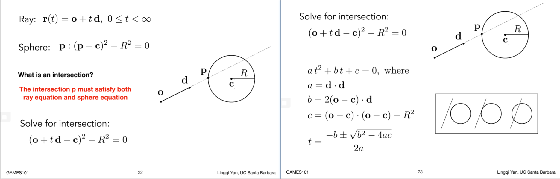
13.2.3.3.1. Ray-Surface Intersection
- Ray Equation
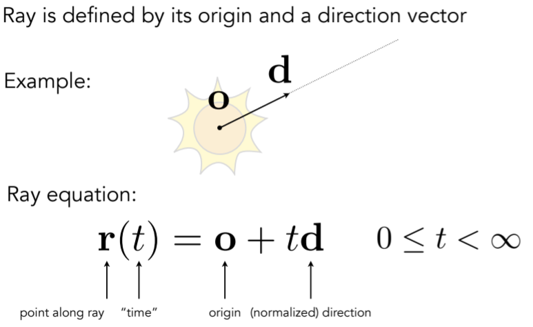
- Ray Intersection With Sphere ,注意这里的t要是正值

- Ray Intersection With Implicit Surface
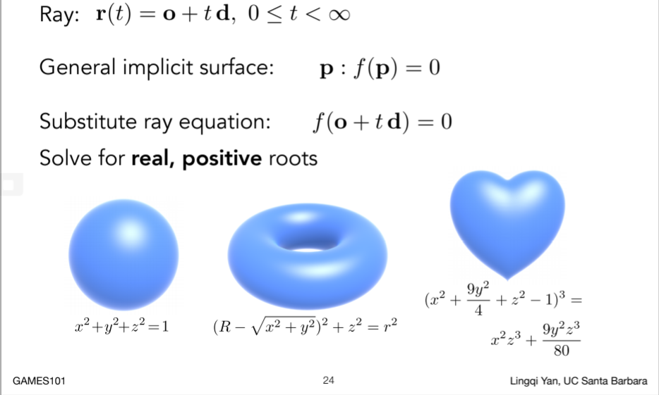
- Ray Intersection With Triangle Mesh

- Why?
- • Rendering: visibility, shadows, lighting …
- • Geometry: inside/outside test :这里一般情况,假如射线在内部,交点奇数,外部偶数
- How to compute? Let’s break this down:
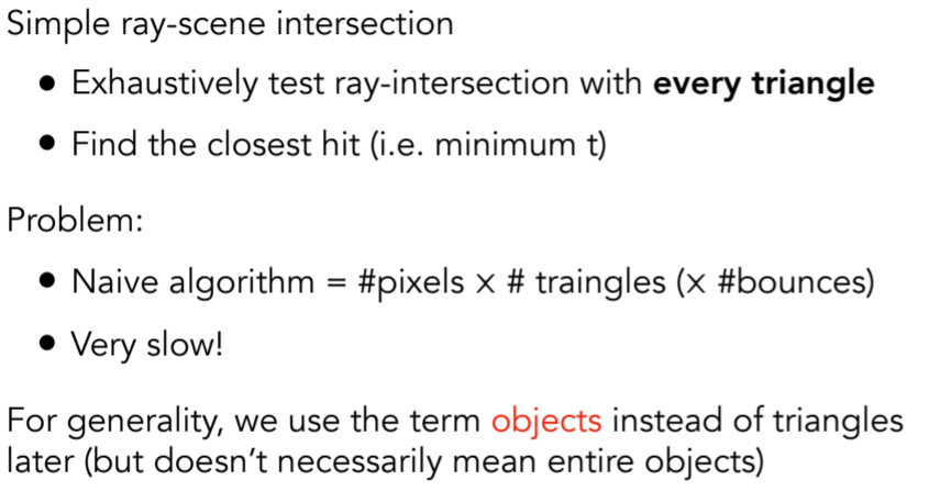
- • Simple idea: just intersect ray with each triangle
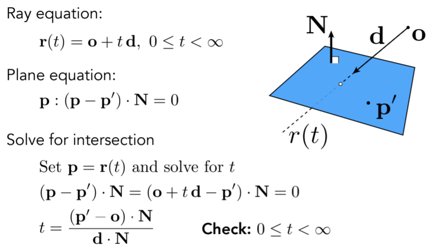
- 解法一:Ray-plane and then inside

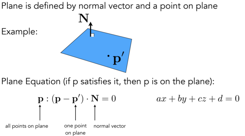
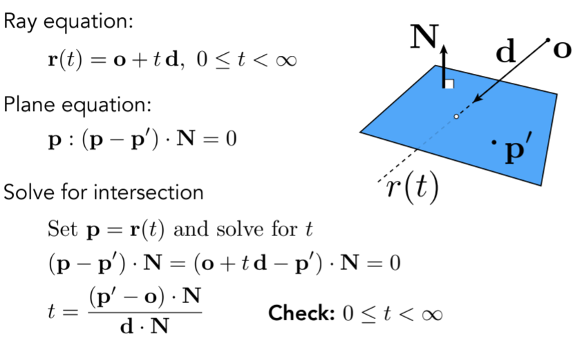
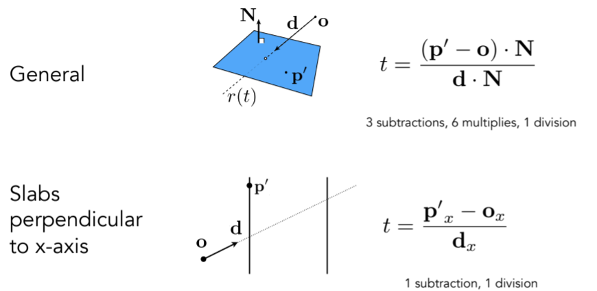
- Plane Equation

- Ray Intersection With Plane
              - 判断inside or not:向量叉乘

            - 解法二:Möller Trumbore Algorithm ,注意这里t b1 b2的隐藏条件

          - • Simple, but slow (acceleration?)

            - Accelerating Ray-Surface Intersection

              - Ray Tracing – Performance Challenges
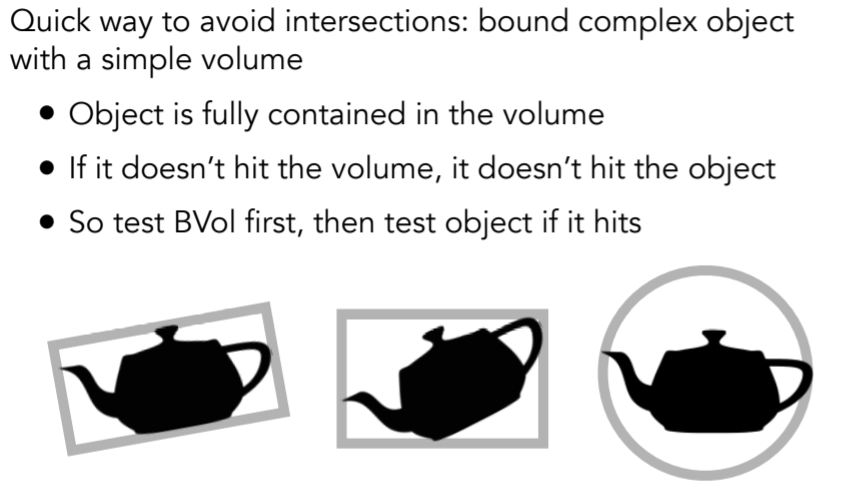
            - Bounding Volumes

              - Bounding Volumes
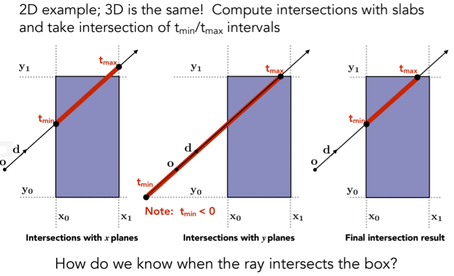
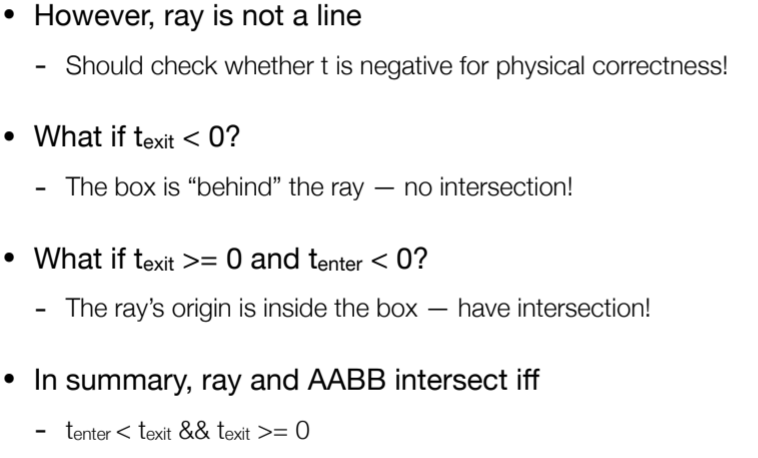
- Ray-Intersection With Box
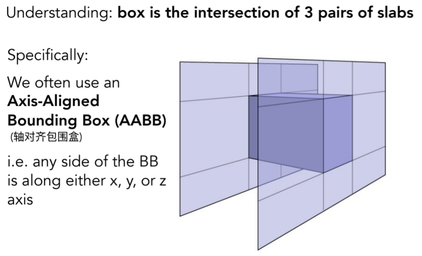
- Ray Intersection with Axis-Aligned Box

- Why Axis-Aligned?
- • Note: can have 0, 1 intersections (ignoring multiple intersections)
14. Lecture 14: Ray Tracing 2(Acceleration & Radiometry)
14.1. Using AABBs to accelerate ray tracing
14.1.1. Uniform Spatial Partitions (Grids)
14.1.1.1. Preprocess – Build Acceleration Grid
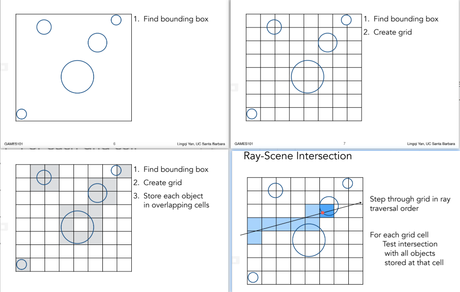
- 这里对于直线的下一个格子寻找,对于该直线,下一个格子的位置要么是右,要么是上
14.1.1.2. problem
14.1.1.2.1. Grid Resolution?

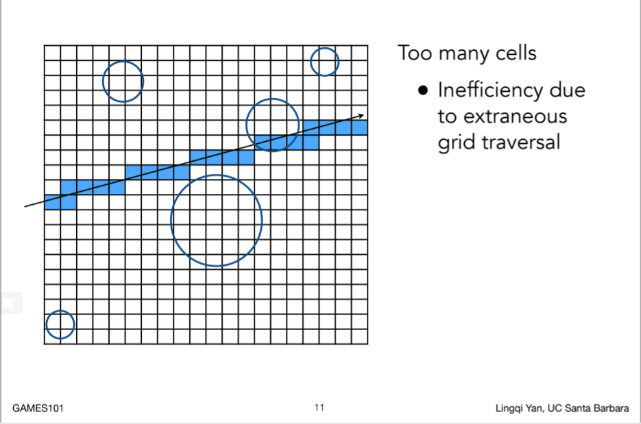
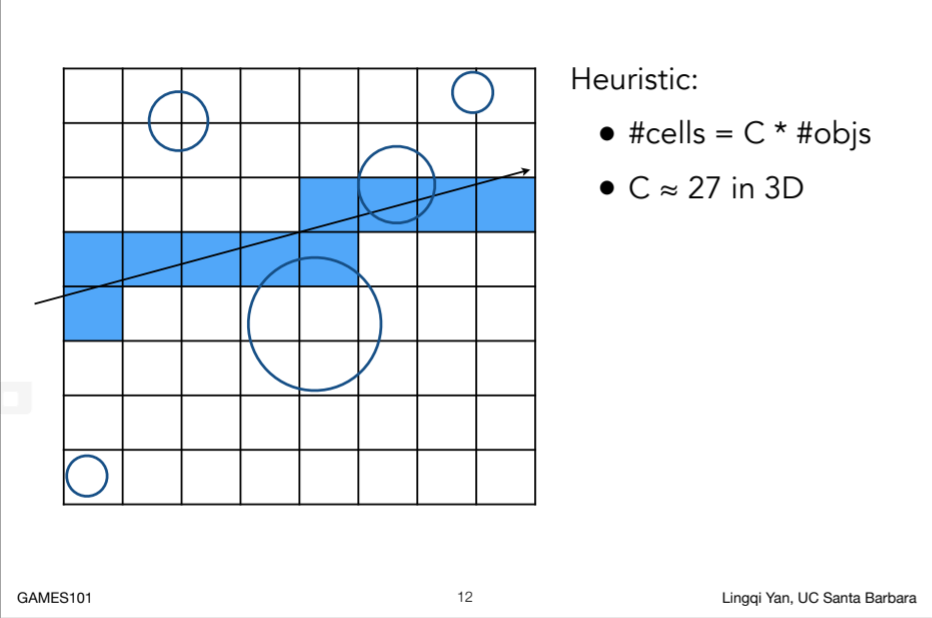
14.1.1.2.2. uniform
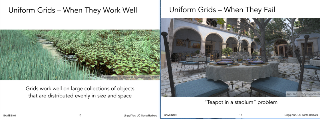
- 对于第二个场景,很多非均匀物体,对于其寻找求交会很慢
14.1.2. Spatial partitions
直观的想法,是不是在稀疏的地方不需要那么密的格子
14.1.2.1. Spatial Partitioning Examples
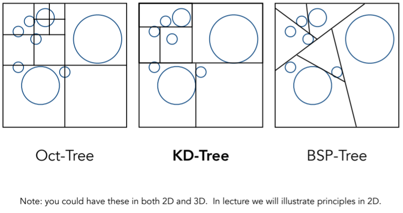
    - 八叉树,跟纬度有关系,在一维下是二叉树,二维如图四叉树,三维下是八叉树,以此类推,更高纬度更多,显然不太好用
    - kd-tree,跟八叉树类似,但是每次只沿着轴向分两块,xy或者xyz交替划分,达到均匀,横平竖直
    - bsp-tree:纬度问题以及不是横平竖直的分割
14.1.2.2. KD-Tree Pre-Processing (这一步骤在光线追踪之前),这里是简化表示,其实每次分割之后,左右都要继续分割,这里只显示每次只分割一半
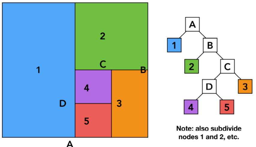
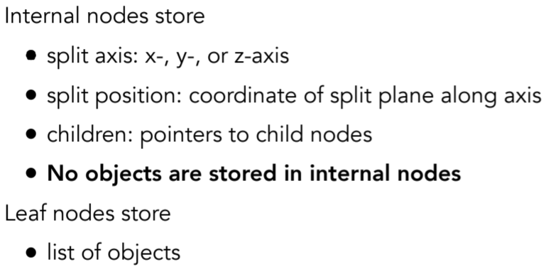
14.1.2.3. Data Structure for KD-Trees ,注意分割方向xyz轴依次,分割不一定是均分,结点包含两个子结点,中间结点不存储物体,只存在叶节点中
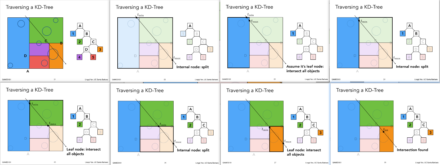
14.1.2.4. Traversing a KD-Tree
14.1.2.5. kd-tree存在的问题
    - aabb与物体的求交判断
    - 物体可能存在与多个aabb中
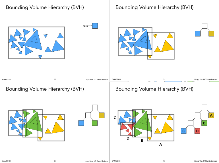
14.1.3. Object Partitions & Bounding Volume Hierarchy (BVH)
14.1.3.1. Bounding Volume Hierarchy (BVH) ,以物体分割为导向,而不是空间分割
14.1.3.2. Summary: Building BVHs
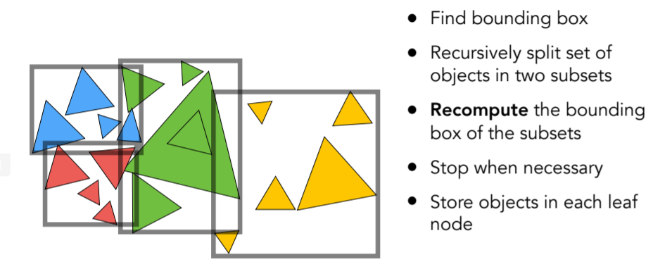
14.1.3.3. Building BVHs 启发式的分割算法,其中第二个目的是让分割的两部分面片数量接近系统,搜索深度相近,快速选择算法
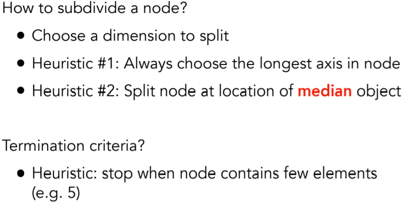
14.1.3.4. Data Structure for BVHs

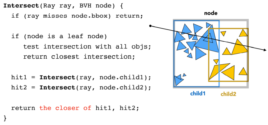
14.1.3.5. BVH Traversal
14.1.3.6. Spatial vs Object Partitions

14.2. Basic radiometry (辐射度量学)
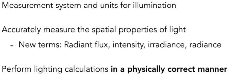
14.2.1. Radiometry — Motivation,主要解决blin-phong模型中的问题,毕竟连单位都没有 ,可以精确地给实际的光下一些物理量的定义
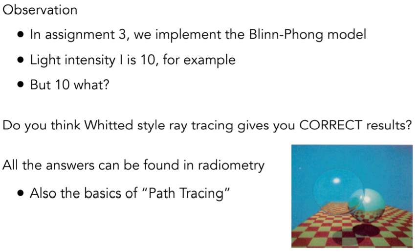
14.2.2. Radiometry:新术语,辐射通量、辐射强度、辐射度、辐射,这里不考虑光的时间属性
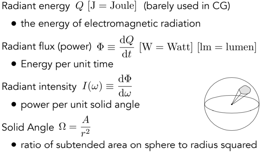
14.2.3. Radiant Energy and Flux (Power)
14.2.3.1. Radiant Energy and Flux (Power) ,注意辐射能量和单位时间内的能量Radiant flux (power)区别,在光学中描述功率用lum描述,也就是描述光有多亮
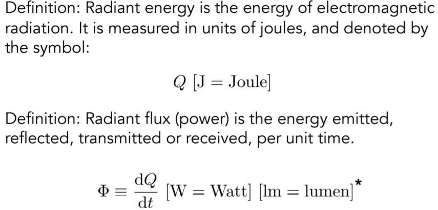
14.2.3.2. Flux – #photons flowing through a sensor in unit time
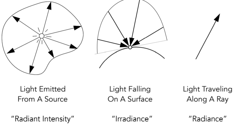
14.2.3.3. Important Light Measurements of Interest ,左:光发出的能量;中:表面接收到的光辐射度;右:光传输过程的辐射
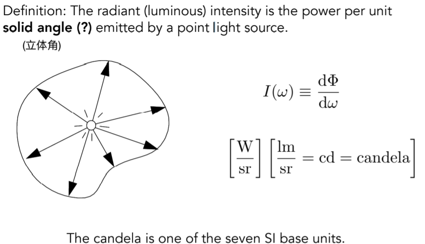
14.2.4. Radiant Intensity
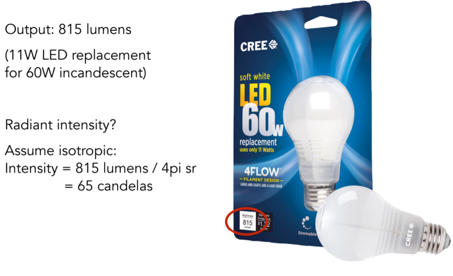
14.2.4.1. Radiant Intensity :立体角,candela是标准单位
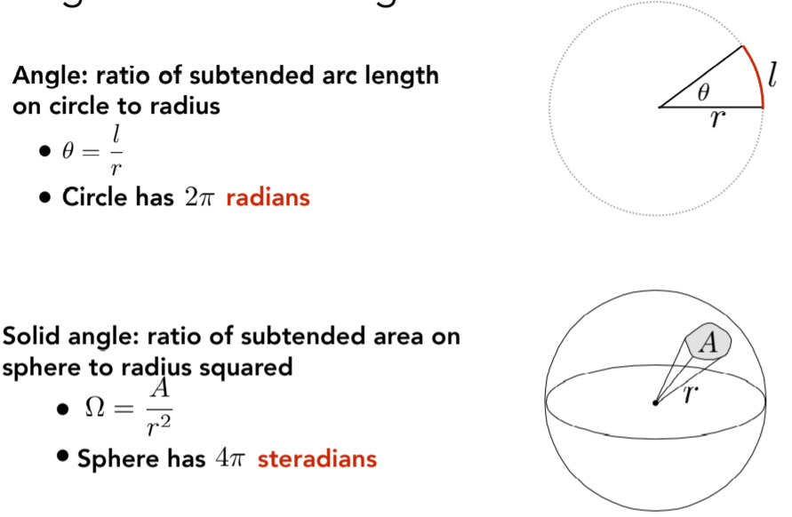
14.2.4.2. Angles and Solid Angles ,类比思想
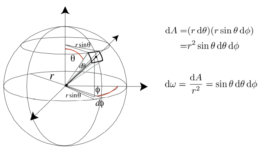
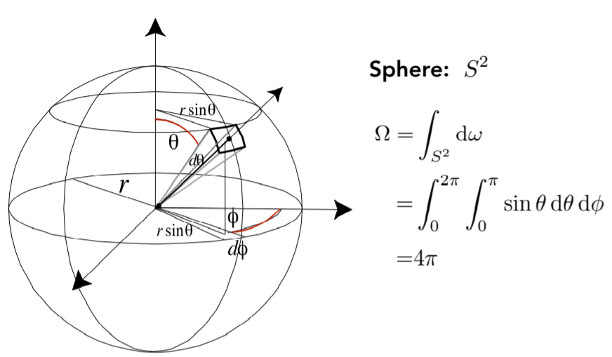
14.2.4.3. Differential Solid Angles 微分立体角
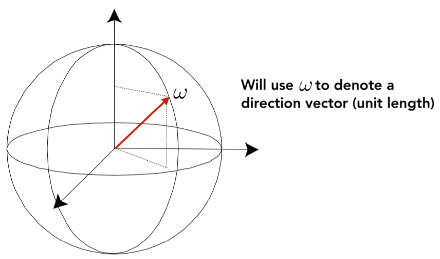
14.2.4.3.1. w as a direction vector ,在光度量中,用w表示一个方向,其实可以theta 和 phi表示
14.2.4.4. Isotropic Point Source 各向同性点源

14.2.4.5. Modern LED Light
15. Lecture 15:Ray Tracing 3 (Light Transport & Global Illumination)
15.1. Radiometry cont.
15.1.1. Reviewing Concepts
后面的概念中,图形学中,说能量的话一般都指的是unit time,不考虑总得能量。尤其是注意这几个概念的区分
15.1.2. Differential Solid Angles 微分立体角

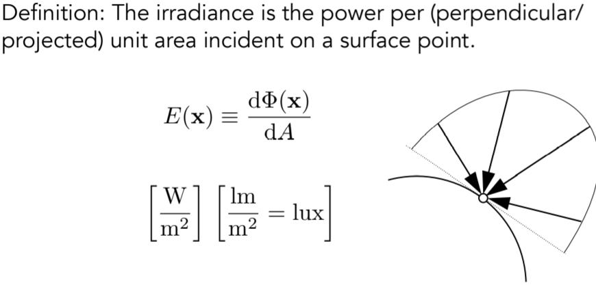
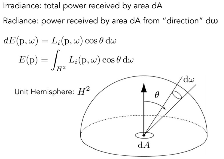
15.1.3. Irradiance
15.1.3.1. Irradiance,注意该处的unit area,必须是与光线垂直的方向,该处是省略了cos theta
15.1.3.1.1. Lambert’s Cosine Law

15.1.3.2. Why Do We Have Seasons?

15.1.3.3. Correction: Irradiance Falloff,注意衰减的是谁,这里不是intensity,因为intensity在传播过程中是不变得。根据intensity的概念,单位立体角,随着r的增加,相应的对应的A也会增大,故intensity不变

15.1.4. Radiance
15.1.4.1. Radiance,描述光传播中的性质

15.1.4.2. Radiance-definition
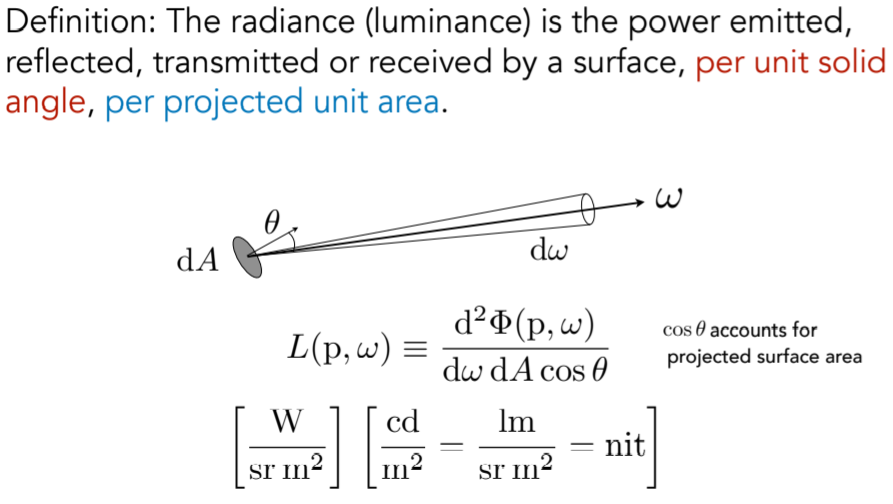
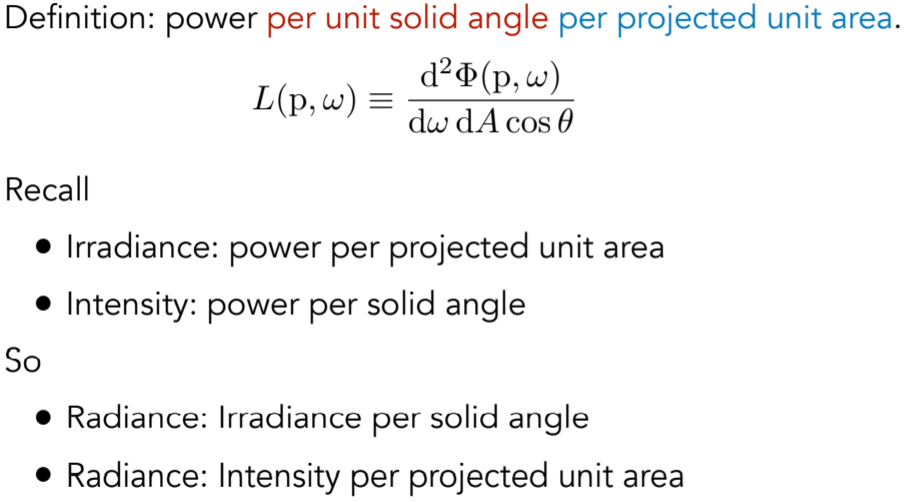
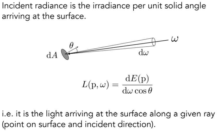
15.1.4.3. Incident Radiance ,联系radiance与irradiance,从w方向上过来的光线打到dA上获得的能量,dw Cos theta是法向上的投影; Irradiance per solid angle ,radiance具有方向性
15.1.4.4. Exiting Radiance,联系intensity与radiance之间的关系,从面dA往一个方向w发出的intensity, Intensity per projected unit area

15.1.4.5. Irradiance vs. Radiance
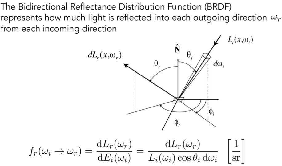
15.2. Light transport (Bidirectional Reflectance Distribution Function (BRDF)双向反射分布函数)
15.2.1. Reflection at a Point: radiance-》irradiance-》radiance
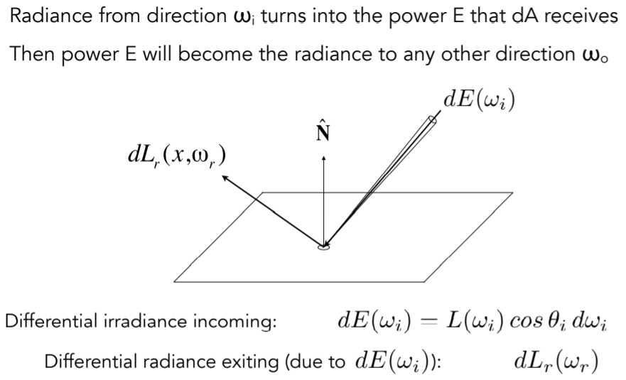
15.2.2. BRDF,从任意一个w入射方向上得到的irradiance是如何分配到各个立体角上的
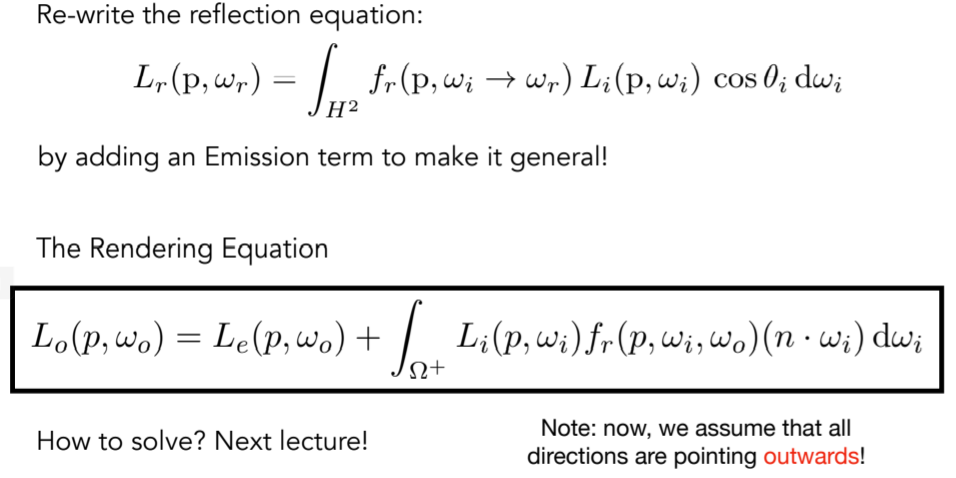
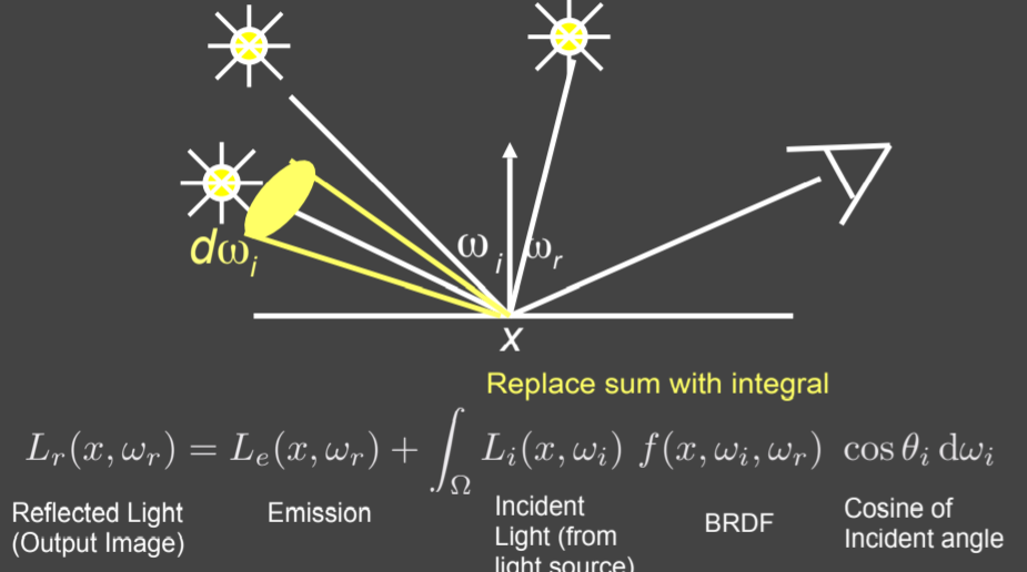
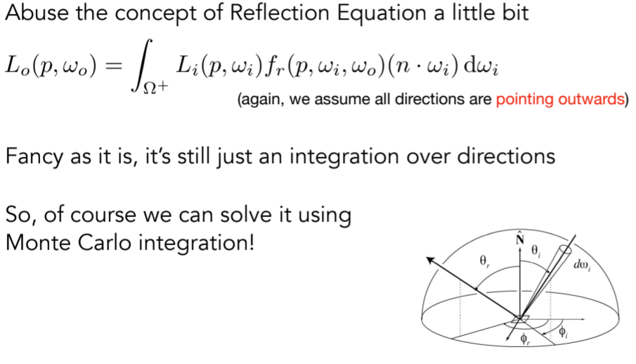
15.2.3. The reflection equation
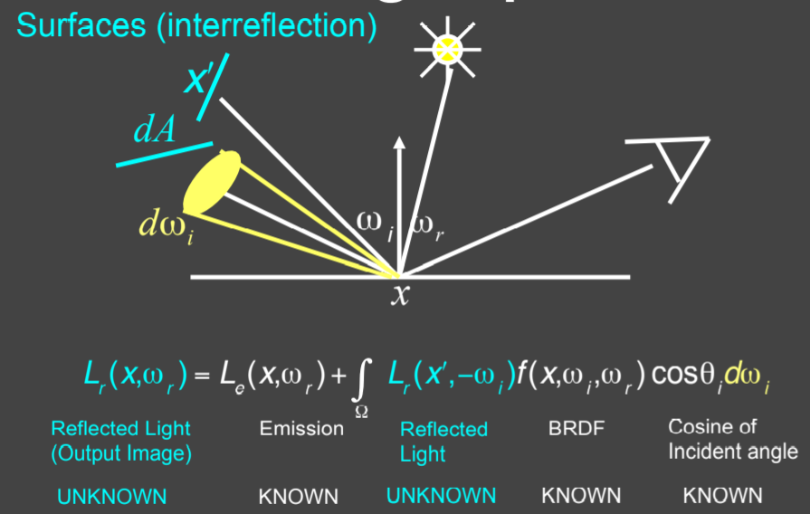
15.2.3.1. The Reflection Equation 对某一个着色点,所有光照(不仅仅包含光源,还包括由点出射的radiance)对观测光线的贡献。任何点的出射radiance都有可能作为其他点的入射radiance。

15.2.3.2. Challenge: Recursive Equation

15.2.4. The rendering equation
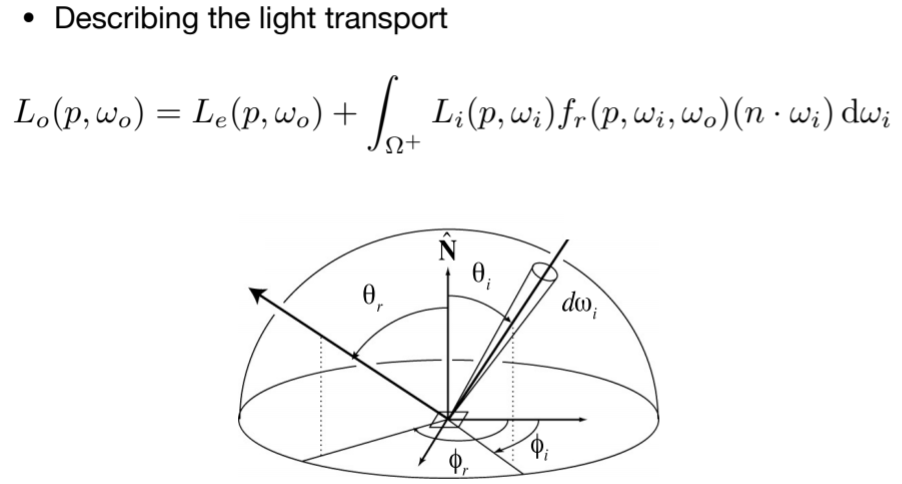
15.2.4.1. The Rendering Equation ,加了自发光项
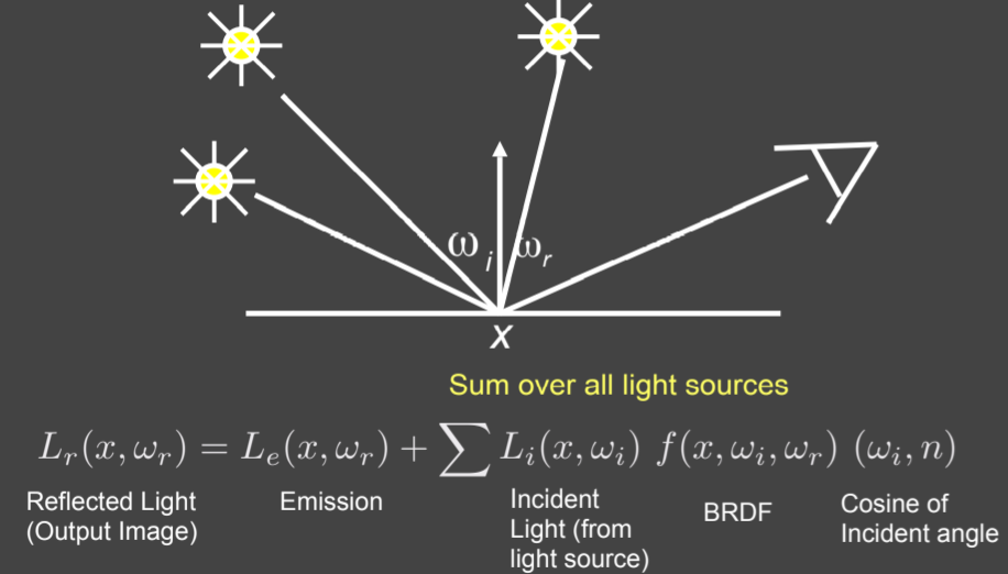
15.2.5. Global illumination:Understanding the rendering equation
15.2.5.1. Reflection Equation
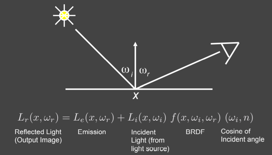
15.2.5.2. Reflection Equation
15.2.5.3. Reflection Equation
15.2.5.4. Rendering Equation
15.2.5.5. Rendering Equation (Kajiya 86)
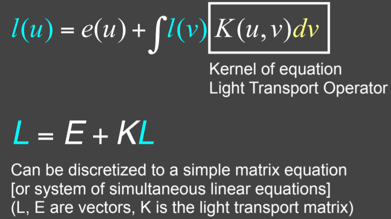
15.2.5.6. Rendering Equation as Integral Equation
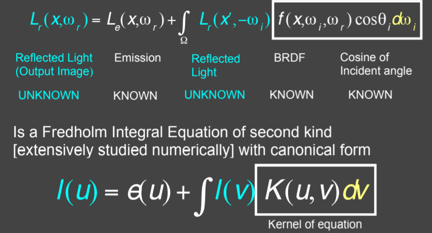
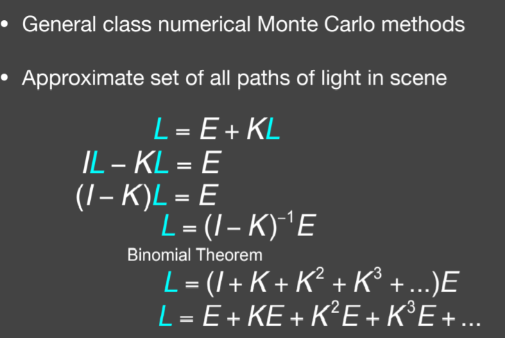
15.2.5.7. Linear Operator Equation
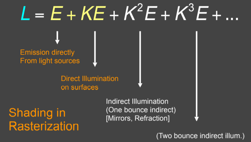
15.2.5.8. Ray Tracing and extensions
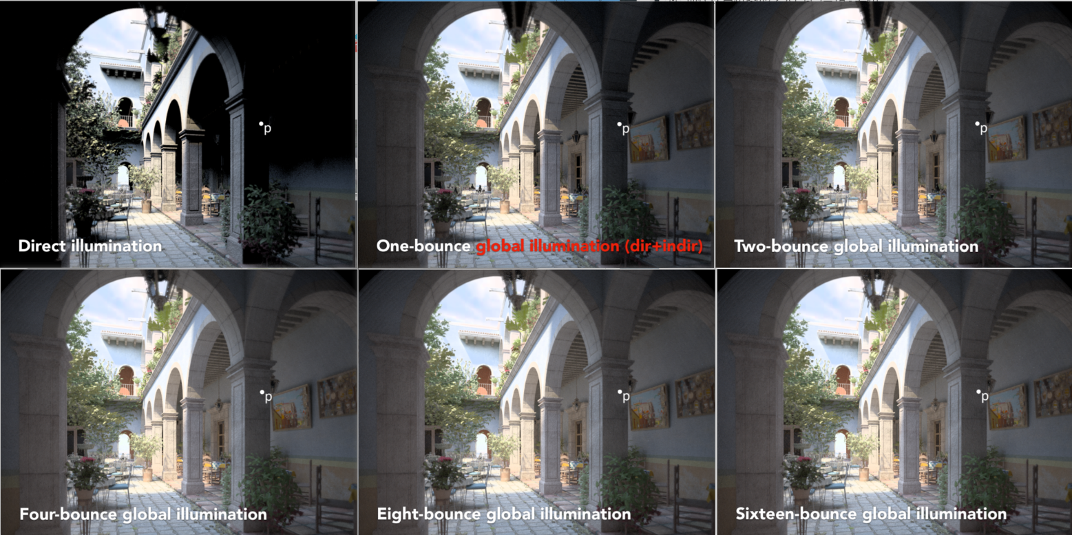
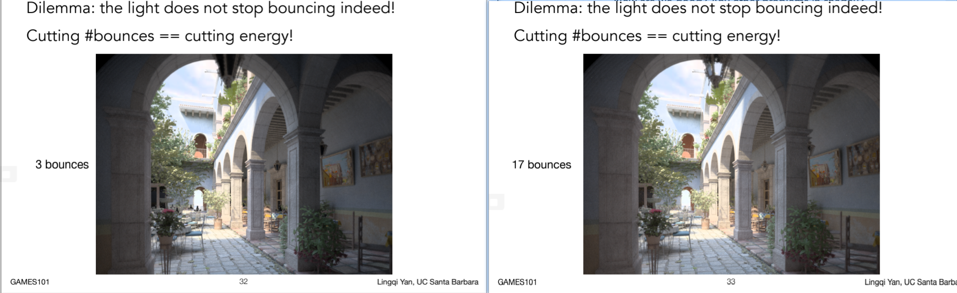
15.2.5.9. Ray Tracing 多次弹射得到的渲染结果
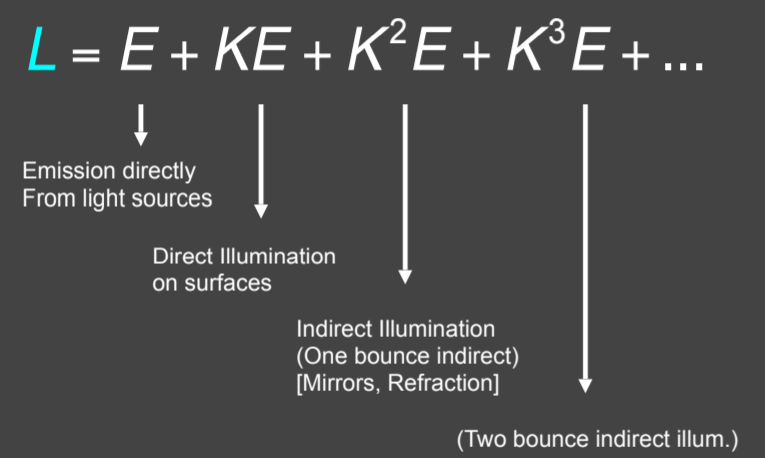
15.2.5.10. 渲染结果
注意观察顶上的灯的变化,这里没太明白,课上是玻璃球需要两次bounce才会出来光线,如果是双层玻璃的,两次弹射进去,再有两次弹射才能出来。这个场景就算加多弹射,最终会收敛,考虑到能量守恒,对于相机一直按着快门的话,则会过曝,因为能量一直在增多
15.3. Probability review
15.3.1. Random Variables
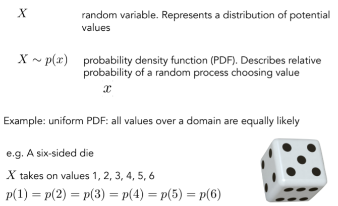
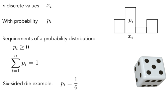
15.3.2. Probabilities
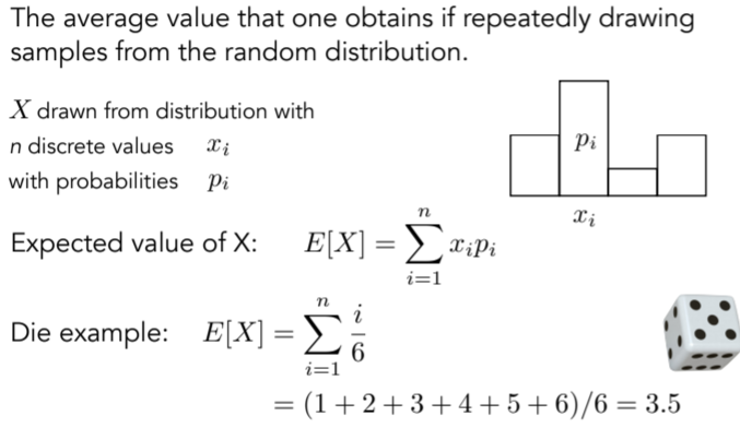
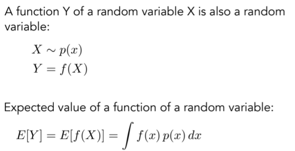
15.3.3. Expected Value of a Random Variable

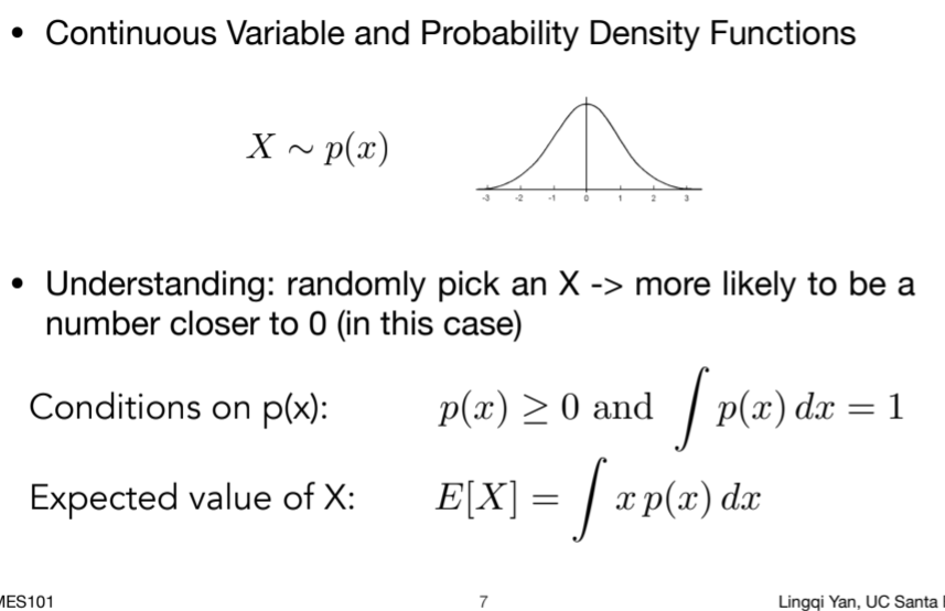
15.3.4. Continuous Case: Probability Distribution Function (PDF)

15.3.5. Function of a Random Variable
16. Lecture 16:Ray Tracing 4(Monte Carlo Path Tracing)
16.1. A Brief Review
16.1.1. Review - The Rendering Equation ,fr是brdf函数
16.1.2. Review - Probabilities
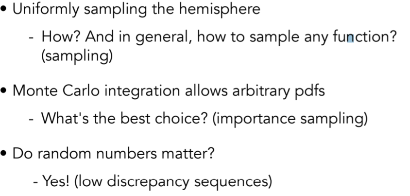
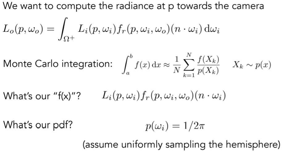
16.2. Monte Carlo Integration
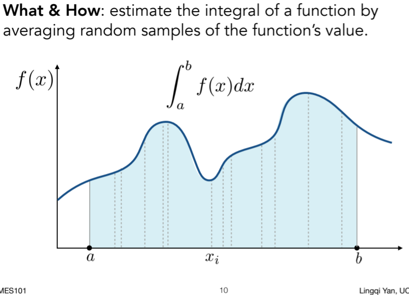
16.2.1. Monte Carlo Integration ,蒙特卡罗积分主要是解决定积分问题,只想要最后求解的数。因为函数的复杂性,有时候不定积分很难求解
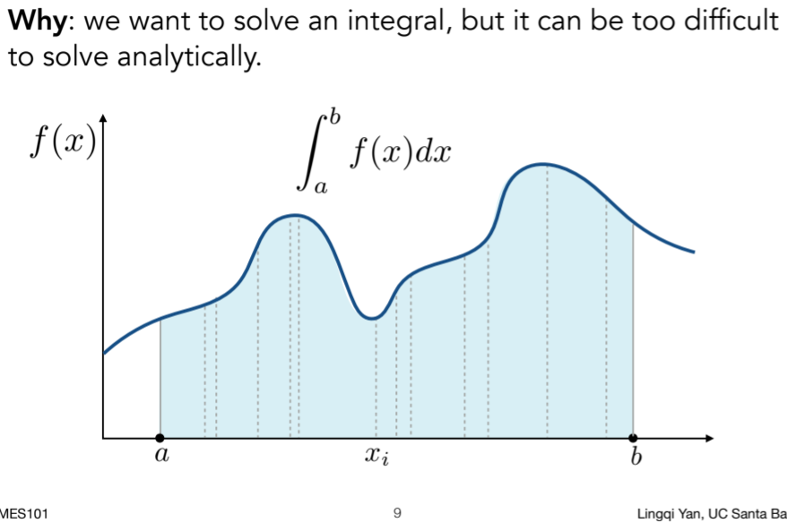

16.2.2. Monte Carlo Integration ,在积分域中采样,得到其对应的值,然后用这个矩形面积近似当前函数的积分结果。为了降低噪声,可以采集n个矩形,再平均。
16.2.3. Monte Carlo Integration
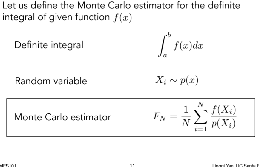
16.2.4. Example: Uniform Monte Carlo Estimator
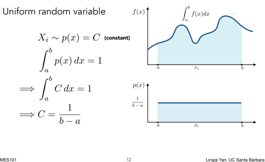
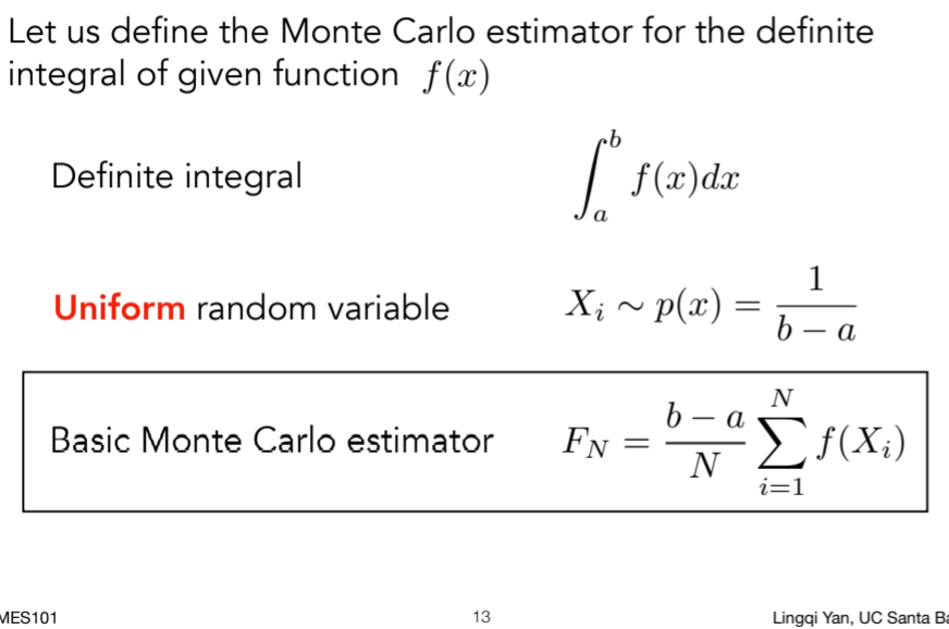
16.2.5. Monte Carlo Integration ,注意采样和积分的域保持一致

16.3. Path Tracing
16.3.1. Motivation: Whitted-Style Ray Tracing
16.3.2. Whitted-Style Ray Tracing: Problem 1
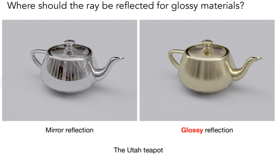
16.3.2.1. mirror reflection,(pure)Specular,完全镜面反射,光射过去一定沿着镜面反射出去。
16.3.2.2. glossy reflection,有镜面的感觉但也有点模糊
16.3.3. Whitted-Style Ray Tracing: Problem 2
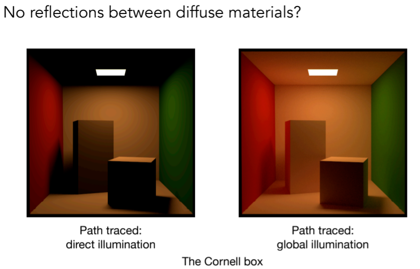
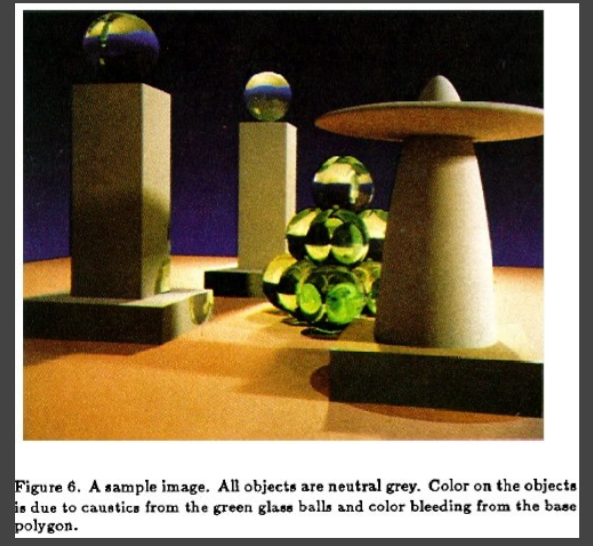
- 右图中,物体上的红色和绿色这种效果称之为color bleeding效果。
16.3.4. Whitted-Style Ray Tracing is Wrong

  - 问题一:积分问题,需要考虑四面八方的光照,因此考虑半球上的光照。
  - 问题二:递归存在
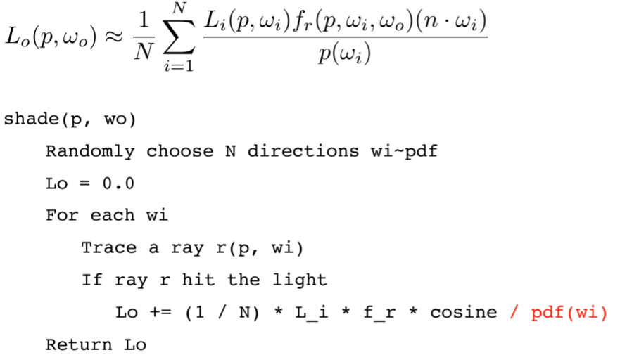
16.3.5. A Simple Monte Carlo Solution
- Wo是观测方向,Wi是各个入射方向,但是图形学中定义都是outwards,因此是方向定义如图
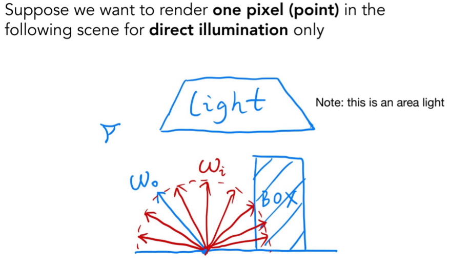
- 写的是反射方程,忽略了自发光项;因为这个也是积分问题,因此可以用蒙特卡罗积分求解
- 3
- 4

- 5
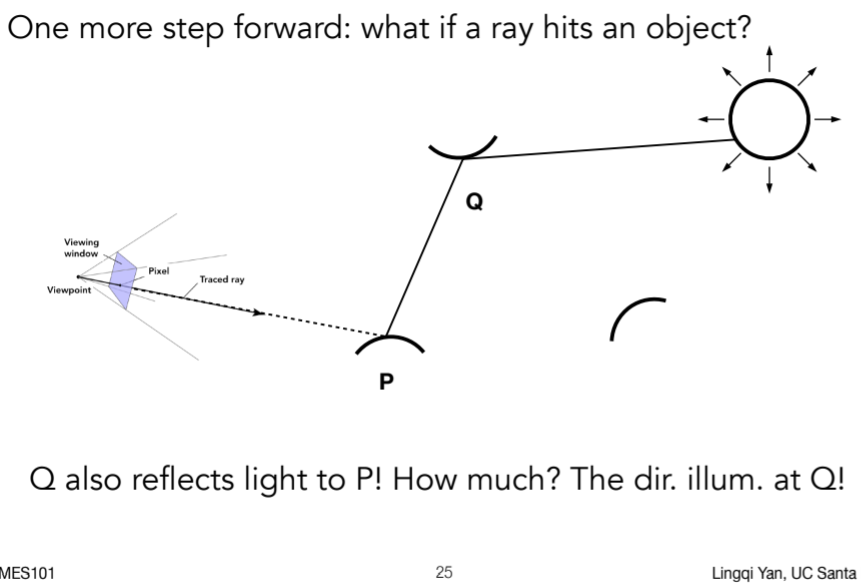
16.3.5.1. Introducing Global Illumination ;这里从Q到P点的radiance是多少呢?类比观测视角,将观测视角放到P点,在P点观测Q点,算Q点的直接光照一样
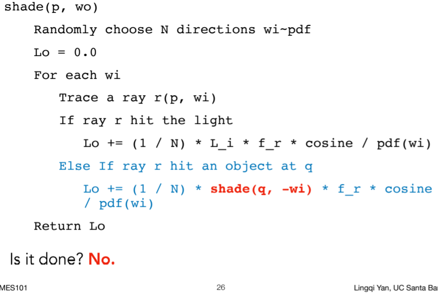
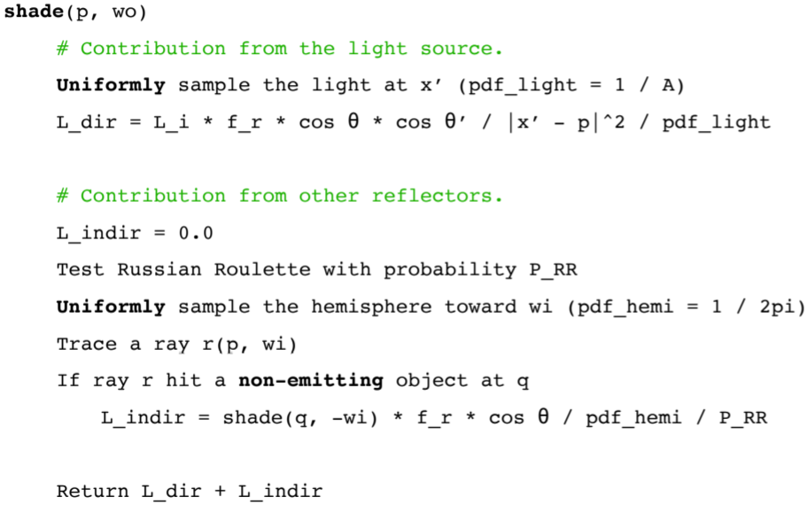
16.3.6. Path Tracing
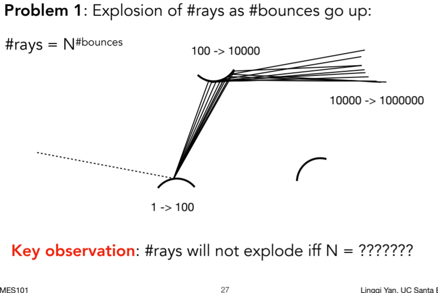
16.3.6.1. Problem 1: Explosion of #rays as #bounces go up: 光线量爆炸,因此将N=1 可以有效解决指数激增问题
16.3.6.1.1. 原因
16.3.6.1.2. 代码,分布式光线追踪 N!=1,N=1时 path tracing

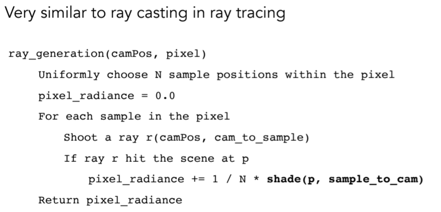
16.3.6.1.3. Ray Generation
- Ray Generation
- Very similar to ray casting in ray tracing
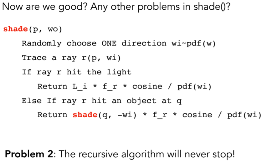
16.3.6.2. Problem 2:The recursive algorithm will never stop!
16.3.6.2.1. 为什么需要终止,实际中光是无数次弹射的,但是计算机图形学中是不允许的,需要有终止
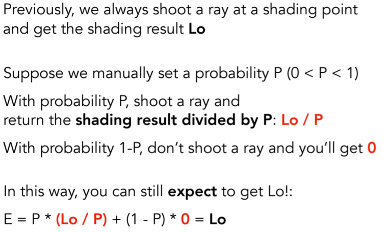
16.3.6.2.2. Solution: Russian Roulette (RR) -俄罗斯轮盘赌
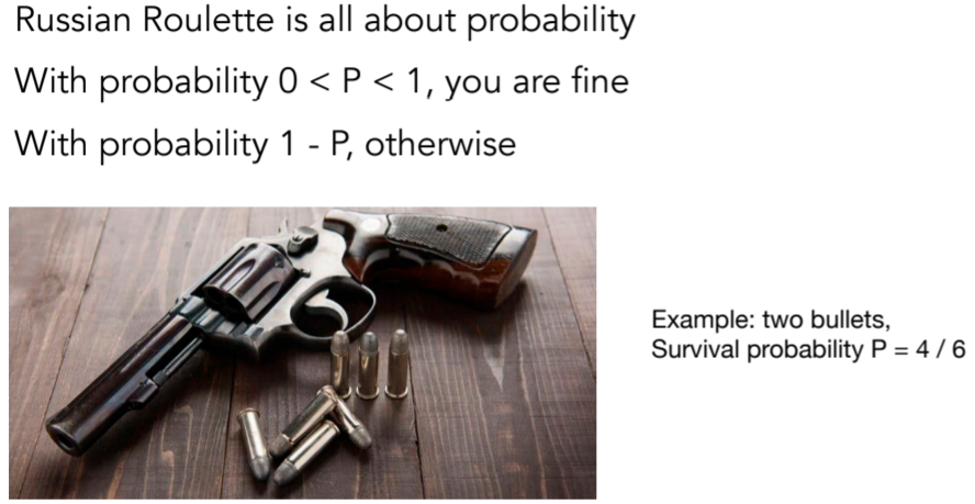
- 原理
- 代码
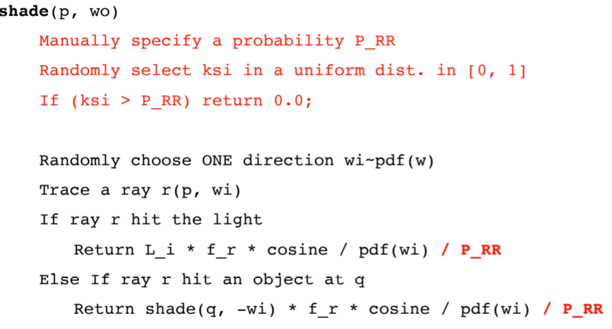

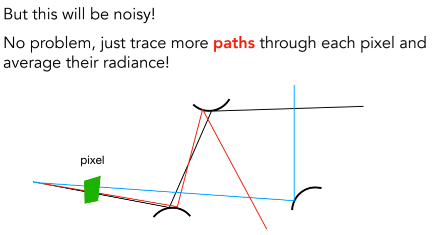
16.3.6.3. Path Tracing ,samples per pixel,就是多少根光线

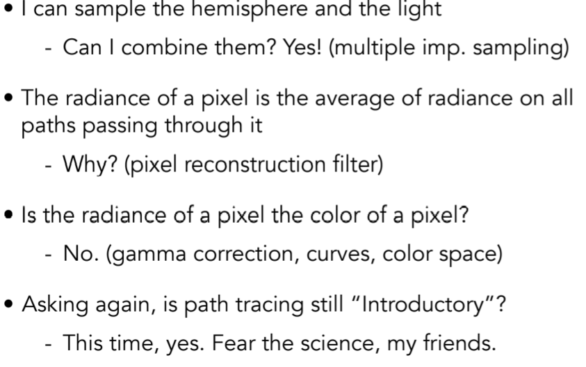
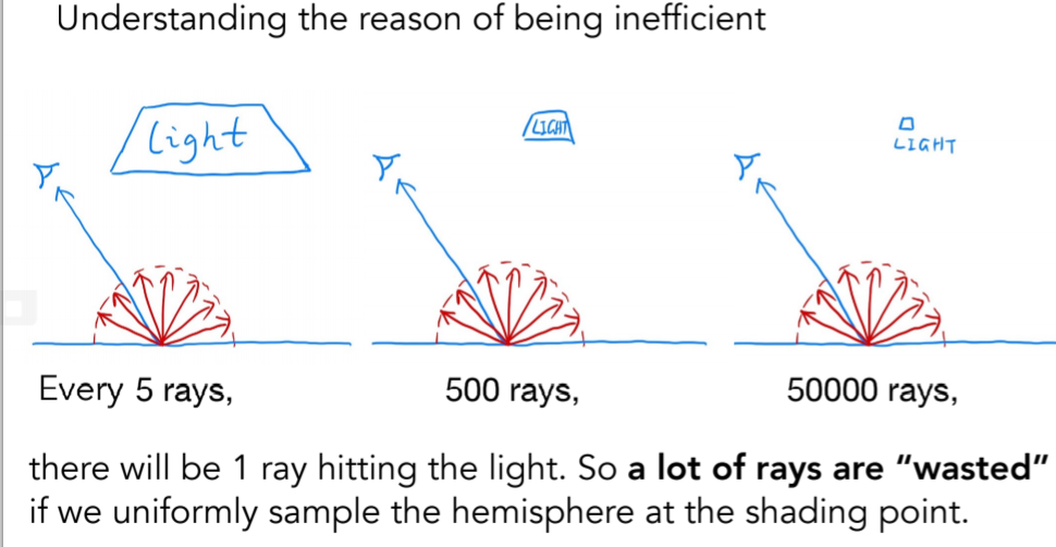
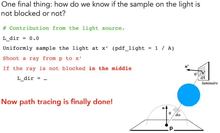
16.3.6.4. Sampling the Light
16.3.6.4.1. Understanding the reason of being inefficient,以往的光线打到光源都是看运气,不合理
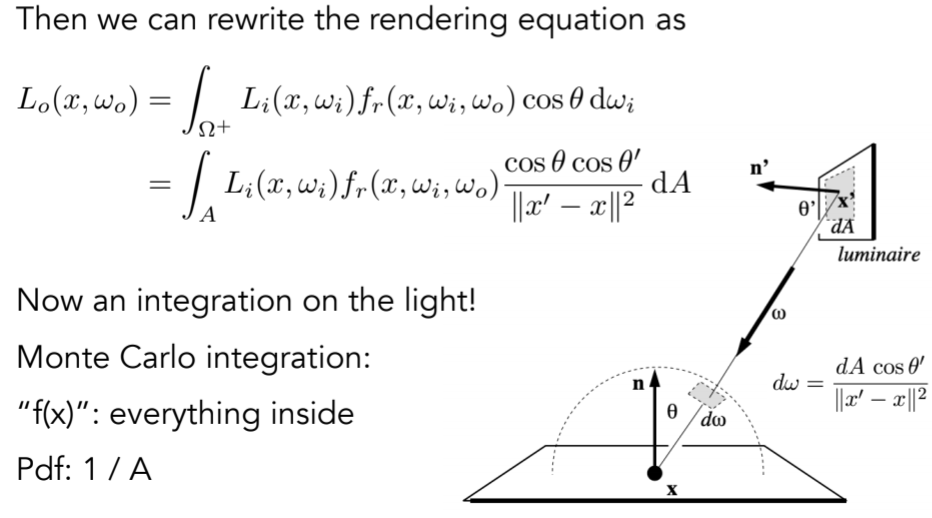
16.3.6.4.2. Sampling the Light (pure math)
注意采用和积分的域一致

16.3.6.4.3. 公式

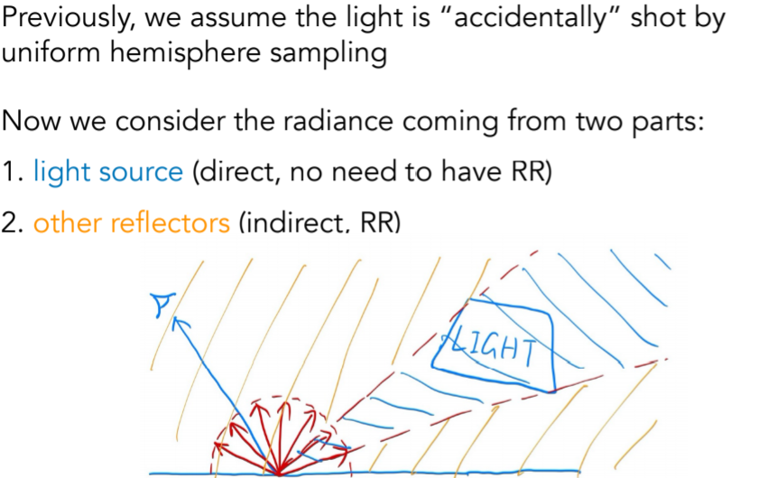
16.3.6.4.4. rendering equation
16.3.6.4.5. radiance coming from two parts
16.3.6.4.6. 代码
16.3.6.4.7. if the sample on the light is not blocked or not?
16.3.7. Some Side Notes
16.3.7.1. Path tracing (PT) is indeed difficult
- Consider it the most challenging in undergrad CS
- Why: physics, probability, calculus, coding
- Learning PT will help you understand deeper in these
16.3.8. Is Path Tracing Correct?

16.3.9. Ray tracing: Previous vs. Modern Concepts
16.3.10. Things we haven’t header-imged / won’t header-img